. 2020 Jun 26;9:e53445. doi: 10.7554/eLife.53445

Figure 3. Characterizing the types of DSTRF variations.

Three types of DSTRF variations are shown over time for three example sites that exhibit each of these types more prominently. The DSTRFs have been masked by 95% significance per jackknifing (n=20). (A) The STRF of the three example sites. (B) Example site E1: Gain change of DSTRF, shown as the time-varying magnitude of the DSTRF at three different time points. Although the overall shape of the spectrotemporal receptive field is the same, its magnitude varies across time. E2: Temporal hold property of an DSTRF, seen as the tuning of this site to a fixed spectrotemporal feature but with shifted latency (lag) in consecutive time frames. E3: Shape change property of DSTRF, seen as the change in the spectrotemporal tuning pattern for different instances of the stimulus. (C) From top to bottom, distribution of gain change, temporal hold, and shape change values for sites in HG and STG. Horizontal lines mark quartiles. Temporal hold and shape change show significantly higher values in the STG.

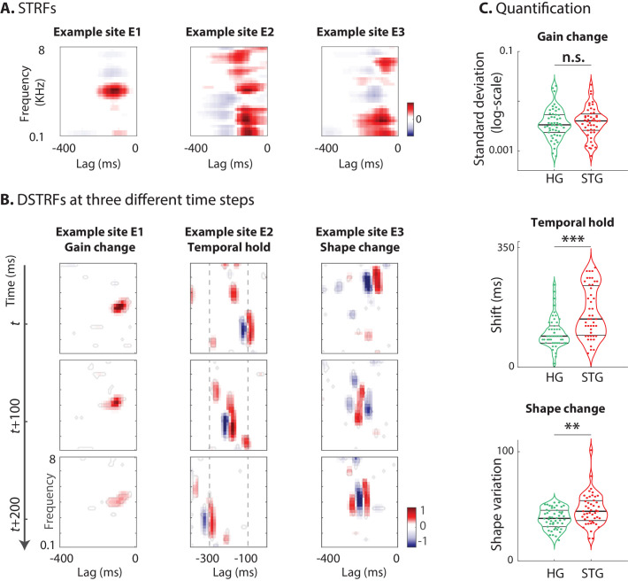
Figure 3—source data 1. A MATLAB file containing three variables, one for each type of quantified nonlinearity — nonlin_gain_change (gain change nonlinearity), nonlin_temporal_hold (temporal hold nonlinearity), nonlin_shape_change (shape change nonlinearity).

Figure 3.

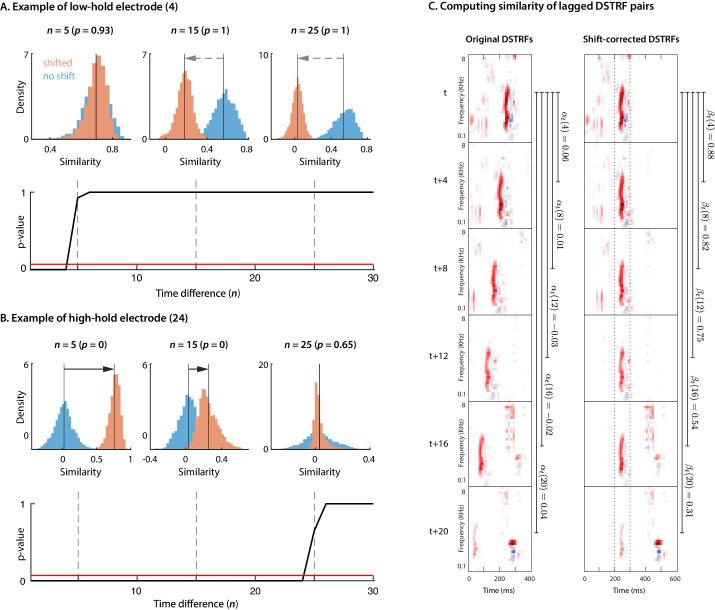
Figure 3—figure supplement 1. Calculating temporal hold.

Figure 3—figure supplement 1.

(A, B) shows the procedure used for calculating temporal hold for two example electrodes. The first row in each panel shows the distributions for DSTRF pair similarities when shifted (βt(n)) and without shift (αt(n)) for all t as described in the methods for three distinct values of time difference between compared DSTRF pairs (n=5,15,25), along with their respective p-values from the one-tailed signed-rank test. The second row shows the p-values for all n30. The red horizontal line indicates the threshold (p=0.05). (C) demonstrates how DSTRF samples are shifted and compared with each other to obtain αt and βt.
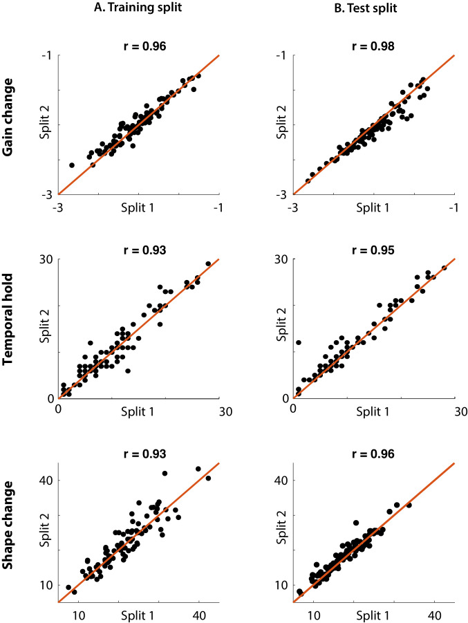
Figure 3—figure supplement 2. Nonlinearity robustness to initialization and data.

Figure 3—figure supplement 2.

(A) We trained 10 instances of the CNN model for each electrode and grouped them into two groups of evens and odds. We measured the three nonlinearity parameters from the average DSTRFs of each group on the test dataset, and compared the values from the two conditions. (B) We measured the three nonlinearity parameters independently from two splits of the test dataset, and compared the values from the two conditions. The R-values represent Spearman correlation.