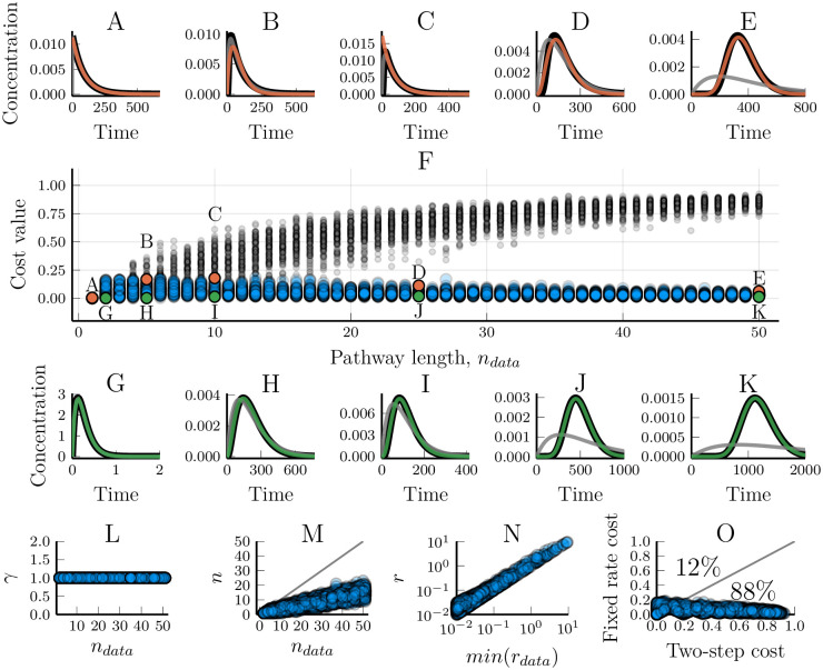
Fig 5. Modelling linear pathways using the fixed-rate assumption for simplification.

The fixed-rate model (Eqs 8 and 9) was fitted towards synthetic data generated by networks of step-lengths varying from 1 to 50. The data sets are the same as those used for Fig 1. (A-E) Examples of the worst model/data fits for the fixed-rate model. Orange lines show simulations of the fitted model and the black line shows the synthetic data. The grey line is the corresponding fit using the two-step truncated model on the same data set. (F) The cost value for models optimised towards 5000 different sets of synthetic data. The x-axis shows the number of steps in the model which were used to generate the data. Blue circles are cost values for the fixed-rate model while grey dots are the cost values for a two-step truncated model. The parameter sets used in figures A-E and G-K are marked accordingly. (G-K) Examples of the best model/data fits. The fixed-rate model (green lines) almost completely matches the data (black lines). (L) The scaling parameter, γ, is accurately identified as 1 in all optimisations. (M) The optimised values of n for different number of steps in the pathway underlying the data. (N) A comparison between the optimised value of r and the smallest rate constant of the model that generated the data. (O) A comparison of the cost values when using either the fixed-rate model or a two-step truncated model to fit the same data. Each circle represents a single synthetic data set. Percentages indicate how many of the data sets had a higher (worse) cost value for the respective models.