Figure 2: Models for time cells.

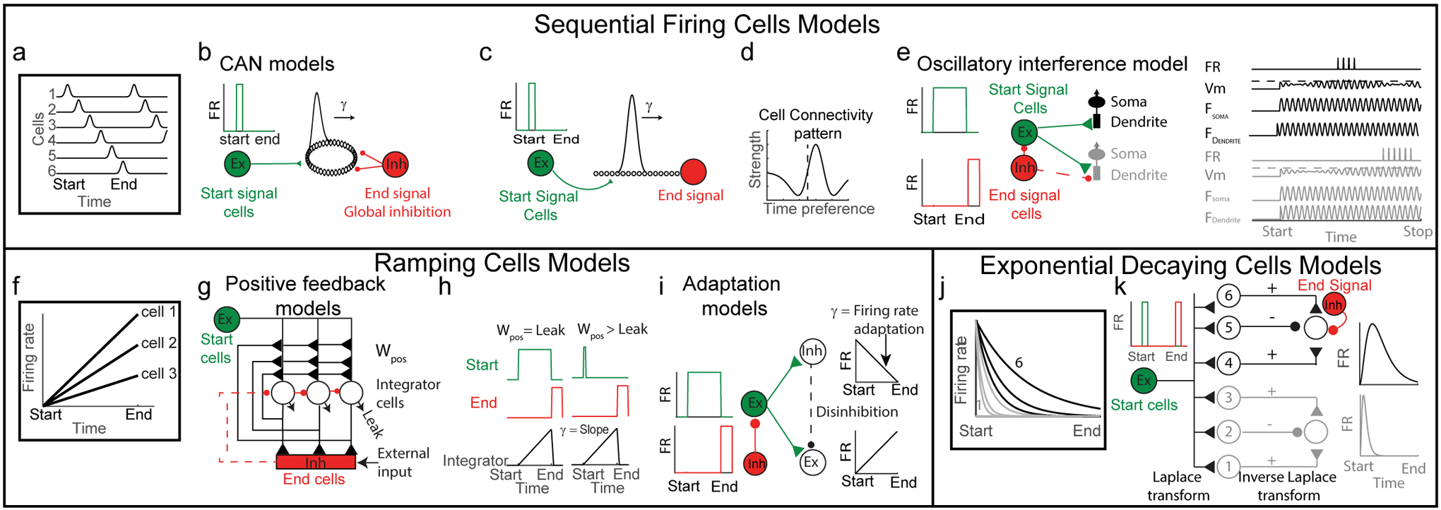
(a) Sequential firing of time cells. Each row represents firing rate (FR) of one cell. Each cell is active at a specific moment within the time interval, and together the sequence of firing cells tiles the entire interval. (b) Ring attractor CAN model. Start population of cells fire a burst at the beginning of the time interval (left, green) and input to a ring attractor (middle, black). Global inhibition provides end signal (right, red). (c) Line attractor CAN model. Start population fire a burst at the beginning of the time interval (left, green) and input to a line attractor (middle, black). End signal is simply cells at the end of the sequence (right, red). (d) Mean connectivity pattern of cells in the CAN model. y-axis represents strength of outgoing weights. x-axis represents time preference of cells that receive the inputs (aligned to the time preference of the output cell at 0, dashed line). (e) Sequence of 2 time cells created by the oscillatory interference model. Start cell fires during the entire interval (top left, green). End signal cell inhibits start cell or integrator cells at the end of the interval (left bottom). On the right a scheme of 2 cells (one in black and one in grey). Each cell excited by a start cell. The dendritic frequency oscillation of each cell (F_dendrite) is different than its somatic frequency oscillation (F_soma, which differs in the 2 cells) and results in an interference pattern (Vm). The membrane potential crosses the firing threshold every beat oscillation. (f) Scheme of 3 ramping cells. Each cell has a different slope. (g) A network model that uses a positive feedback mechanism to integrate inputs over time and generate ramping cells. All integrator cells receive feedforward input from start cells (green). Output integrator cells (black) are connected by recurrent excitation and also send excitation to end neurons. End cells (red) inhibit integrator cells once the rate of inputs they receive crosses a threshold or by external input. Adapted from (Seung et al. 2000). (h) Activity of each cell type (start cells: green; end cells: red; integrator cells: black) when recurrent excitation is equal to the leak current (left, W_pos > Leak). or when recurrent excitation is slightly higher than the leak current (right, W_pos > Leak). (i) A model network generating ramping activity by an adaptation process. A population of excitatory persistent firing cells (fire at a constant rate during the time interval) excite a population of inhibitory (Inh) and excitatory (Ex) neurons. Due to adaptation of the firing rate in the inhibitory neurons, their firing rate decreases. This disinhibits the excitatory population, which in turn increases their firing rate, which creates a ramping firing pattern. Adapted from (Reutimann et al. 2004). (j) Exponentially decaying firing rates of 6 cells with different time constants in response to a start burst, analogous to the Laplace transform of a delta function (a start burst). (k) Start cells (green) give a pulse input to a cell population with exponentially decaying firing rates, each with different time constants (the cells arranged according to their time constants in increasing order bottom to top). The exponentially decaying cell population projects to the output layer cells (on the right) through center-off surround-on connectivity pattern. Thus, each cell in the output layer receives a weighted sum of several exponential decaying cells, implementing an inverse Laplace transform, which in turn produces time cells in the output layer (Howard et al. 2014; Liu et al. 2019).