Figure - PMC

Skip to main content

An official website of the United States government

Here's how you know

Here's how you know

Official websites use .gov
A .gov website belongs to an official government organization in the United States.

Secure .gov websites use HTTPS
A lock ( ) or https:// means you've safely connected to the .gov website. Share sensitive information only on official, secure websites.

View full-text article in PMC

. 2020 Jul 16;140:110074. doi: 10.1016/j.chaos.2020.110074

Search in PMC
Search in PubMed
View in NLM Catalog
Add to search

© 2020 Elsevier Ltd. All rights reserved.

Since January 2020 Elsevier has created a COVID-19 resource centre with free information in English and Mandarin on the novel coronavirus COVID-19. The COVID-19 resource centre is hosted on Elsevier Connect, the company's public news and information website. Elsevier hereby grants permission to make all its COVID-19-related research that is available on the COVID-19 resource centre - including this research content - immediately available in PubMed Central and other publicly funded repositories, such as the WHO COVID database with rights for unrestricted research re-use and analyses in any form or by any means with acknowledgement of the original source. These permissions are granted for free by Elsevier for as long as the COVID-19 resource centre remains active.

PMC Copyright notice

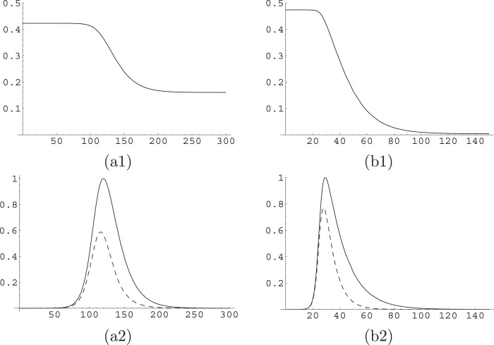
Fig. 2 — Dynamics of x(t) in the A-SIR model. We plot x(t) in upper plots (a1) and (b1); and I(t) (dashed curve) and J(t) (solid curve) in lower plots (a2) and (b2). These are considered along the solutions of the A-SIR model for $α = 1.13 * 10^{- 8},$ $β = 1 / 7,$ $η = 1 / 14,$ and $ξ = 1 / 10$ ; in the left column, i.e. in plots (a1) and (a2), with $S_{0} = 2 * 10^{7}$ and $I_{0} + J_{0} = 10$ ; in the right column, i.e. in plots (b1) and (b2), for $S_{0} = 6 * 10^{7}$ and $I_{0} + J_{0} = 30$ . The scale of plots (a2) and (b2) is chosen so that the maximum of J(t) is at level one.