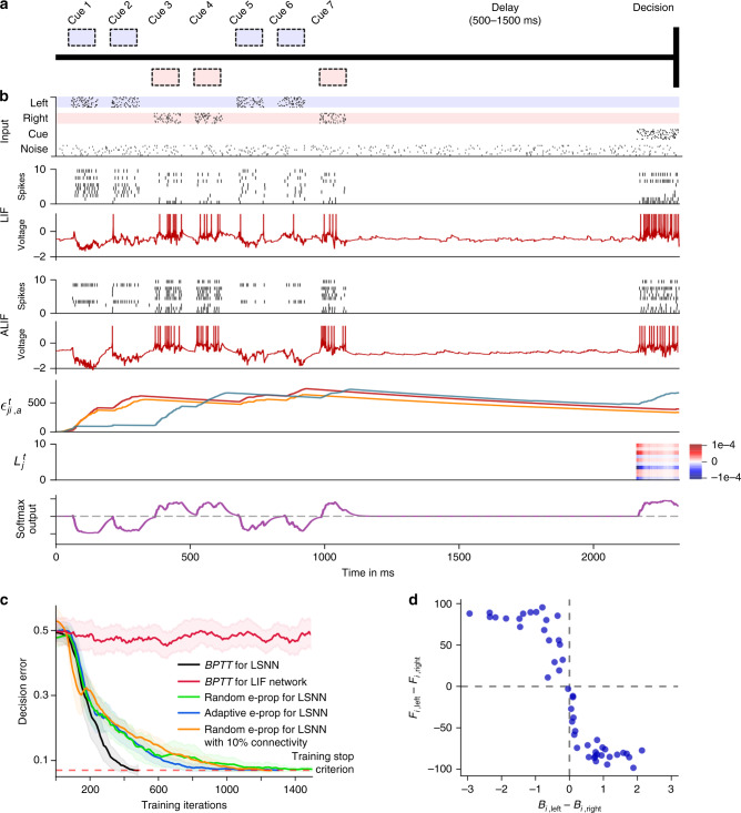
Fig. 3. Solving a task with difficult temporal credit assignment.

a Setup of corresponding rodent experiments of ref. ²³ and ref. ¹⁴, see Supplmentary Movie 1. b Input spikes, spiking activity of 10 out of 50 sample LIF neurons and 10 out of 50 sample ALIF neurons, membrane potentials (more precisely: $v_j^t-A_j^t$) for two sample neurons j, three samples of slow components of eligibility traces, sample learning signals for 10 neurons and softmax network output. c Learning curves for BPTT and two e-prop versions applied to LSNNs, and BPTT applied to an RSNN without adapting neurons (red curve). Orange curve shows learning performance of e-prop for a sparsely connected LSNN, consisting of excitatory and inhibitory neurons (Dale's law obeyed). The shaded areas are the 95% confidence intervals of the mean accuracy computed with 20 runs. d Correlation between the randomly drawn broadcast weights B_jk for k =  left/right for learning signals in random e-prop and resulting sensitivity to left and right input components after learning. f_j,left (f_j,right) was the resulting average firing rate of neuron j during presentation of left (right) cues after learning.