

Abstract
This short note constructs Mobility Zones to facilitate the discussion on the geographic extent of individual mobility restrictions to control the spread of Covid-19. Mobility Zones are disjoint sets of counties where a given level of individual mobility directly or indirectly connects all counties within each set. I compute Mobility Zones for the United States and each state using smartphone-based mobility data between counties. The average area and population of Mobility Zones have sharply shrunk around the onset of the epidemic. Pre-Covid-19 Mobility Zones may be useful in calibrating quantitative studies of targeted restriction policies, or for policymakers deciding on the adoption of specific mobility measures. Two examples suggest the use of Mobility Zones to inform within-state differences and cross-state coordination in mobility restriction policies.
Keywords: Individual mobility, Covid-19, Social distancing, Lockdown policies
Graphical abstract
Highlights
-
•
The geographic spread of Covid-19 depends on the extent of individual mobility.
-
•
Lockdown and reopening policies are determined at the local and state level.
-
•
Cell phone data identify areas of contagion spread under no mobility restrictions.
-
•
I construct partitions of U.S. and its states that vary with mobility intensity.
-
•
These partitions inform within- and across-state lockdown and reopening decisions.
1. Introduction
The current pandemic of Covid-19 has induced a large number of countries to restrict individuals’ mobility and production activities to limit the diffusion of the virus, with massive economic damage. As policymakers consider how to lift and perhaps reimpose these restrictions, it is essential to measure which sets of places are connected by individual mobility in normal, unrestricted circumstances. Widely used SIR models (Kermack and McKendrick, 1927) postulate that the spread of the contagion is a function of the contact rate between individuals. If a path of strong enough mobility ordinarily connects two distant locations, policymakers might consider them as part of the same area for lockdown decisions. On the other hand, policymakers might temper restrictions, and economic damage, in some subset of unaffected locations if most individual mobility occurs within that same area.
This note identifies Mobility Zones (MZs) for the United States and individual states. MZs are disjoint sets of counties where a given level of individual mobility directly or indirectly connects all counties within each set. The average population size of these MZs sharply shrinks around the onset of the epidemic, plausibly reflecting endogenous social distancing (e.g. Toxvaerd, 2020) and compliance with stay-at-home orders. In the United States, most decisions about mobility restrictions are under the responsibility of individual states. I then compute pre-Covid-19 MZs to identify areas that are connected by individual mobility in ordinary times. Two examples suggest the use of Mobility Zones to inform within-state differences and cross-state coordination in mobility restriction policies.
To construct these zones, we see counties as nodes of a network. Our working assumption is that the contagion can travel directly between two counties only when they are linked. An edge links two counties if individuals’ mobility between them is above a given threshold in the interval . We then partition the network of the economy into components. Counties are part of the same component if there is a sequence of links, or path, that connects them in the network. A county only belongs to one component, and all counties are assigned to some component (see e.g. Jackson, 2008, sec. 2.1.5 for a formal definition of the component of a network). For an economy , we term a component of this network a Mobility Zone (MZ) at level , or . By varying the mobility threshold between zero and one, the set of MZs varies in general from a singleton (the whole economy) to the set of all the counties in the economy considered.
We implement this procedure empirically with the daily location exposure (LEX) indices made publicly available by Couture, Dingel, Green, Handbury, and Williams (2020a) - henceforth, Couture et al. (2020a). These indices are based on data from smartphones “pinging” in a given location and date. For a given day , the data reports, among all the phones active in county , the fraction of phones that have also been active in a location at least once in the previous fourteen days. Each day, from January 20, 2020, the data provide a square matrix of values for 2018 U.S. counties with a sufficient number of active devices. We take these indices as proxies for individual mobility.
There is an already rich literature on the current Covid-19 pandemic. Related to this note, Goldfaber and Tucker (2020) use mobile devices data to study which kind of retail outlets generated most social interactions. Fang et al. (2020) quantify the effect of limits on individual mobility on the spread of the virus in Wuhan, and Harris (2020) shows evidence that the subway facilitated the spread in New York. Kuchler et al. (2020) show that infections correlate with social interactions as measured by social media ties. In general, MZs may help calibrate future research on optimal lockdown and restriction-lifting policies. Current research on these questions includes Acemoglu et al. (2020), Alvarez et al. (2020), Fajgelbaum et al. (2020), Jones et al. (2020), or Rampini (2020). MZs parallel the widely used Commuting Zones in Tolbert and Sizer (1996). Commuting zones are aggregates of counties based on commuting patterns; two counties must have commuting ties if they are in the same commuting zone. MZs are based on individual mobility for any purpose; two counties must be connected by a path (but may or may not have direct links) if they are in the same MZ. Counties-to-MZs correspondences are available at any threshold of county-to-county mobility.
2. Methodology
Denote with the set of locations in the economy. is left implicit whenever it is not necessary. For a given day , Couture et al. (2020a) reports, among all the phones active in a geographic unit , the fraction of phones that have also been active in a location at least once in the previous fourteen days, . I construct an undirected adjacency matrix representing the economy as follows.
First, for each pair , compute the average
| (1) |
When describing the evolution of MZs over time (Fig. 1, Fig. 2), is each day from January 20, 2020 to May 5, 2020, and . When computing the pre-Covid-19 MZs (for the remaining figures), is the set of days in the three weeks from Monday, January 20, 2020, to Sunday, February 9, 2020. Considering all days in a week allows accounting for within-week variation in mobility patterns. These three weeks are the longest period of data that appears reasonably unaffected by the Covid-19 outbreak, as discussed below.
Fig. 1.

Average population in the daily MZs for the U.S., (left) and (right).
Fig. 2.

Average population in the daily MZs for California, (left) and (right).
Each belongs to the interval . As a second step, for a fixed interaction threshold , compute
| (2) |
as an indicator variable equal to 1 if this average share is greater than or equal to , and otherwise.
I say that and are linked at level if or , or both. As a third step, I construct an symmetric matrix that indicates if any two counties are linked at level .
represents the adjacency matrix of an undirected network for . As a fourth step, I identify all the components of this network using readily available computer routines.
3. Mobility zones: Discussion
I start by constructing daily MZs for the United States economy at various mobility thresholds . Fig. 1 reports the average daily MZ population over time for and . These values of are chosen purely for illustrative purposes. Dashed lines mark different weeks. Individual mobility results in a stable MZ average size until, roughly, 2/17. The data reveals a slight increase in the average population size of counties connected by individual mobility after that date, likely a seasonal pattern (Couture et al., 2020b p. 19). A sharp decrease appears to start approximately in coincidence with the U.S. Government declaration of the State of National Emergency, on 3/13 (solid blue line). The average MZ size drop as much as 60%–65% of the Pre-Covid-19 period. As of May 5, the average size of MZ is still about 30%–40% lower than the beginning of the sample period. These patterns of a slight increase and then a sharp decrease in size are found for most thresholds and both average population and average land size of MZs.
Fig. 2 reproduces the same statistics when daily MZs are computed for California only. California is the first state to issue a shelter-in-place order for seven counties on 3/16,2 and it imposes a state-wide order on 3/19. The reduction in the average size of the MZs is consistent with broad compliance with the order.
Mobility Zones appear to reasonably capture the consequences of individual mobility choices. We then ask, which groups of counties are connected by individual mobility in unrestricted circumstances? This information can be useful in future quantitative research on geographically targeted lockdowns, and for policymakers evaluating re-openings or planning for new restrictions. From both perspectives, policymakers might need to synchronize lockdown policies within an MZ; however, they might not need to do it across MZs.
To answer this question, I compute pre-Covid-19 MZs using the average data between 1/20/2020 and 2/9/2020, three full weeks of data. Given the evidence in Fig. 1, this conservatively short period appears unaffected by changes in individual mobility. Correspondences between counties and MZs for a fine grid of are made available for the U.S. and individual states.
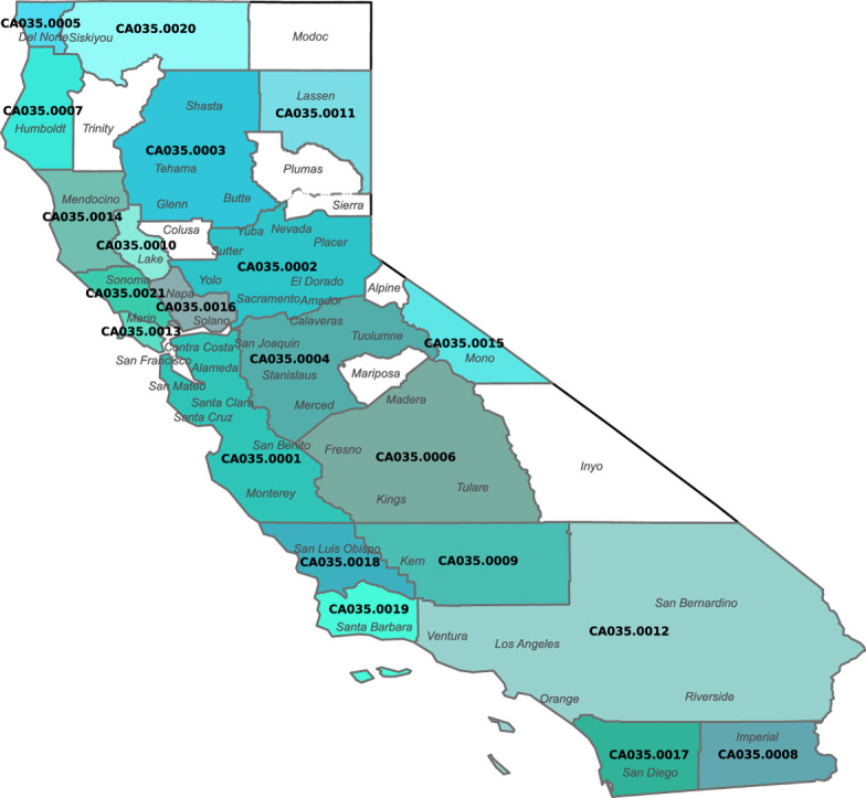
Fig. 3 shows, for the state of California, two MZ maps, for mobility thresholds equal to (left) and (right); in our notation, and . Each color corresponds to a distinct MZ (white areas have no data in Couture et al., 2020a). The code of the MZ, in Italic in the maps, is comprised of the geographical area of reference (“CA”), the threshold used in percentage points (020 or 035), and a four-digit progressive identifier. The maps also report the county names.
Fig. 3.

Mobility zones for California, (left) and (right).
As one might expect, most pairs of counties do not have connections at such high levels. These values of are already around the th–96th percentiles of mobility in the data for California. Nonetheless, paths can form between counties that are relatively far. For example, individual mobility generates paths from Monterrey to San Francisco (at ) or up to the Northern end of the state (at ). These considerations are compatible with statewide stay-at-home orders that include counties with limited initial infection rates.
Reducing the mobility threshold for a direct “link” between two counties naturally shrinks the number of MZs and it increases their size. At , the Bay area becomes part of a larger MZ including most of the north of the state. More in general, Fig. 4 plots the number of MZs for California as a function of the interaction threshold. The evaluation of restriction policies may be framed in terms of what is the appropriate value of , and considering the associated MZs.
Fig. 4.

Mobility zones as a function of the mobility threshold.
These maps can be generalized to compute MZs for the whole United States at once. MZs can cross state boundaries. Fig. 5 shows the map for . Again, white areas appear where data is not available. Quite naturally, distinct MZs appear around large metropolitan areas like New York. More interestingly, large MZs also appear cutting across Alabama, Georgia, and South Carolina, or in the Great Lakes region. An appropriately determined may indicate the need for coordination across states in optimally lifting or reimposing mobility restrictions.
Fig. 5.

Mobility zones for the U.S. economy, .
4. Limitations and conclusions
In this note I construct Mobility Zones, disjoint sets of counties where a given level of individual mobility directly or indirectly connects all counties within each set. MZs reveal a significant change in individual mobility throughout the epidemic. I compute MZs for a pre-Covid-19 period, which may prove useful to calibrate quantitative research on geographically targeted lockdown policies and to support discussion around the extent of mobility restrictions. This geographical dimension enters the broader debate on the trade-off between heavier economic costs and higher chances of further waves of infections. Two examples illustrate the use of MZs to inform within-state differences and cross-state coordination in mobility restriction policies. A state-to-state aggregation of mobility data could inform policy coordination across states when only state-wide restrictions are available. I focus on the United States, but a similar intuition can be applied to other countries wherever comparable data is available.
Some caveats and limitations of this work need to be discussed. First, this note does not advocate for any particular value of the threshold , a decision best left to epidemiologists and policymakers. Second, as Couture et al. (2020a) emphasize, the indices used are a “proxy” for individual mobility, but they do not fully capture individual mobility. Hence, the extent of these areas needs to be carefully considered, even if one knows the optimal . Third, these mobility indices reflect pre-Covid-19 patterns in the early part of the year. As such, they may not fully capture natural mobility patterns occurring at the time of the year when restrictions are lifted or reimposed. Fourth, both mobility in an area and the local impact of a policy may be influenced by policies in adjacent mobility zones.
Footnotes
These are the counties of Alameda, Contra Costa, Marin, Santa Clara, San Francisco, San Mateo and Santa Cruz.
References
- Acemoglu, D., Chernozhukov, V., Werning, I., Whinston, M.D., 2020. A Multi-Risk SIR Model with Optimally Targeted Lockdown. NBER Working Paper 27102.
- Alvarez, F., Argente, D., Lippi, F., 2020. A Simple Planning Problem for COVID-19 Lockdown. NBER Working Paper 26981.
- Couture V., Dingel J., Green A., Handbury J., Williams K. 2020. Location exposure index based on PlaceIQ data, mimeograph. [Google Scholar]
- Couture V., Dingel J., Green A., Handbury J., Williams K. 2020. Measuring movement and social contact with smartphone data: a real-time application to COVID-19, mimeograph. [DOI] [PMC free article] [PubMed] [Google Scholar]
- Fajgelbaum, P., Khandelwal, A., Kim, W., Mantovani, C., Schaal, E., 2020. Optimal Lockdown in a Commuting Network. NBER Working Paper 27441.
- Fang, H., Wang, L., Yang, Y., 2020. Human Mobility Restrictions and the Spread of the Novel Coronavirus (2019-nCoV) in China. NBER Working Paper 26906. [DOI] [PMC free article] [PubMed]
- Goldfaber, A., Tucker, C., 2020. Which Retail Outlets Generate the Most Physical Interactions? NBER Working Paper 27042.
- Harris, J., 2020. The Subways Seeded the Massive Coronavirus Epidemic in New York City. NBER Working Paper No. 27021.
- Jackson M. Princeton University Press; 2008. Social and Economic Network. [Google Scholar]
- Jones, C., Philippon, T., Venkateswaran, V., 2020. Optimal Mitigation Policies in a Pandemic: Social Distancing and Working from Home. NBER Working Paper 26984.
- Kermack W.O., McKendrick A.G. A contribution to the mathematical theory of epidemics, part I. Proc. R. Soc. Lond. Ser. A. 1927;115(772):700–721. [Google Scholar]
- Kuchler, T., Russel, D., Stroebel, J., 2020. The Geographic Spread of COVID-19 Correlates with Structure of Social Networks as Measured by Facebook. NBER Working Paper No. 26990. [DOI] [PMC free article] [PubMed]
- Rampini, A., 2020. Sequential Lifting of COVID-19 Interventions with Population Heterogeneity. NBER Working Paper No. 27063.
- Tolbert, C., Sizer, M., 1996. U.S. Commuting Zones and Labor Market Areas - A 1990 Update. Economic Research Service Staff Paper 9614, U.S. Department of Agriculture.
- Toxvaerd, F.M.O., 2020. Equilibrium Social Distancing. Cambridge Working Papers in Economics 2021.