Figure 3.

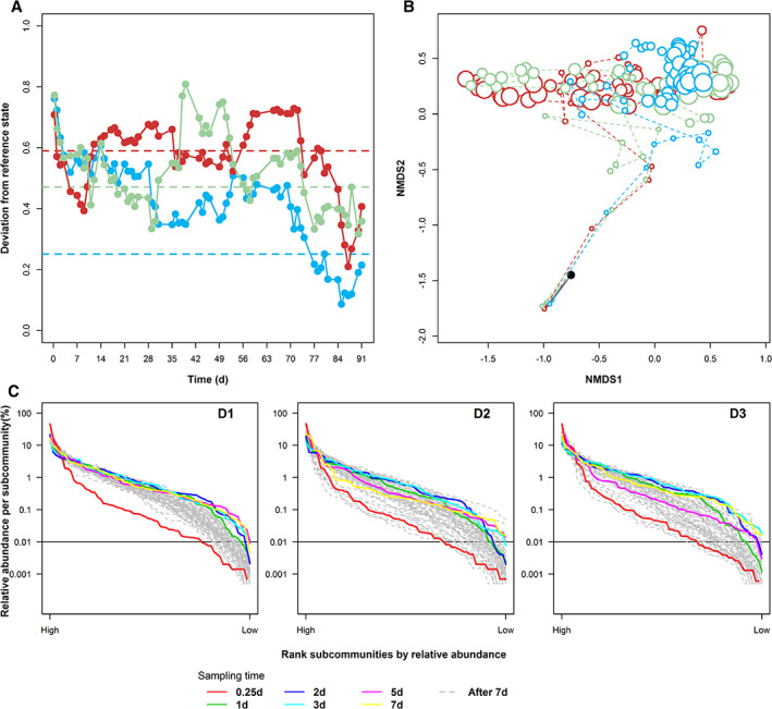
Community analysis based on all subcommunities in samples of disturbed reactors D1, D2 and D3. A. The boundary of the reference space was calculated using the last 10 time points (79–91 days). The reference state was determined by calculating the mean values per subcommunity of these 10 samples. The pairwise deviations between the reference state and successive samples were estimated as Canberra distances (D1: blue, D: red and D3: green). The maximum value of deviation from the reference state was chosen as the boundary of reference space per reactor (dashed line). B. Dissimilarity analysis of community structures per reactor. Each point on the nMDS plot represented a community sample (inoculum: black, D1: blue, D2: red and D3: green). The sampling time is represented increasing point sizes. c: Rank‐order abundance curves of samples from reactors D1 (left), D2 (middle) and D3 (right); all 68 subcommunities per sample were ranked according to their relative cell abundances and displayed in decreasing order from left to right. The horizontal line marks the height of relative cell abundance at 0.01%. The slopes of samples at 0.25 day (red line) are D1: −0.054, D2: −0.055 and D3: −0.056; mean values of slopes after the adaptation (grey lines) are D1: −0.049, D2: −0.049 and D3: −0.052.