Modeling and forecasting the spread and death rate of coronavirus (COVID-19) in the world using time series models

Abstract

Coronaviruses are a huge family of viruses that affect neurological, gastrointestinal, hepatic and respiratory systems. The numbers of confirmed cases are increased daily in different countries, especially in Unites State America, Spain, Italy, Germany, China, Iran, South Korea and others. The spread of the COVID-19 has many dangers and needs strict special plans and policies. Therefore, to consider the plans and policies, the predicting and forecasting the future confirmed cases are critical. The time series models are useful to model data that are gathered and indexed by time. Symmetry of error's distribution is an essential condition in classical time series. But there exist cases in the real practical world that assumption of symmetric distribution of the error terms is not satisfactory. In our methodology, the distribution of the error has been considered to be two-piece scale mixtures of normal (TP–SMN). The proposed time series models works well than ordinary Gaussian and symmetry models (especially for COVID-19 datasets), and were fitted initially to the historical COVID-19 datasets. Then, the time series that has the best fit to each of the dataset is selected. Finally, the selected models are applied to predict the number of confirmed cases and the death rate of COVID-19 in the world.

1. Introduction

Coronaviruses are a huge family of viruses that affect neurological, gastrointestinal, hepatic and respiratory systems. This family can be grown among humans, bats, mice, livestock, birds, and others [1], [2], [3]. In 2003, a type of coronavirus, called SARS coronavirus (SARS-CoV), was distributed from animal to animal [4]. In 2012, another type of coronavirus, named as MERS coronavirus (MERS-CoV), was significantly distributed from human to human [4]. Late in year 2019, the World Health Organization (WHO) reported many cases in China with respiratory diseases. It was verified that most of the reported cases contacted with the persons that had went to a seafood market in Wuhan [5]. Recently, a new type of coronavirus, named COVID-19 (it may be also named 2019-nCoV), is spreading in Wuhan [6]. The scientists believe that the COVID-19 acts in human similar to that are in bats. However, to know the main source of the COVID-19, more scientific studies are needed. Based on the reports, the COVID-19 has been observed in others cities in China and also in about other 198 countries (up to 06 February 2020). The Centers for Disease Control and Prevention (CDC) verified that the COVID-19 is distributed from human to human. Based on the CDC's reports, the COVID-19 is spread by touching surfaces, close contact, air, or objects that contain viral particles. The COVID-19 is a dangerous virus, because the incubation period of the COVID-19 is at least 14 days [7], and it can spread to others in the incubation period. A recent research indicates that the median age and incubation period of confirmed cases are respectively 3 days and 47.0 years [8].

The number of confirmed cases has increased daily in different countries, specially in United State American, Italy, Spanish, Germany, Iran, China and other countries. The spread of the COVID-19 has many dangers and needs strict special plans and policies. Therefore, to consider the plans and policies, the prediction and forecasting the future confirmed cases are critical. The number of the unreported COVID-19 cases in China has been mathematically estimated by [9]. Using a data-driven analysis, they estimated that there are 469 unreported COVID-19 cases in China in 1–15 January 2020. Based on the information of some Japanese passengers in Wuhan, Nishiura et al. [10] estimated the rate of the infection for COVID-19 in Wuhan. The results indicated a rate of 9.5% for infection and a rate from 0.3% to 0.6%, for death. Since the size of the considered population is very small, there is doubt in about accuracy of estimated rates. Based on a mathematical model, Tang et al. [11] concluded that the transmission risk of COVID-19 is averagely about 6.47 persons and predicted the time that the peak of COVID-19 will be reached. Using the information of 47 patients, Thompson [12] estimated a sustained human-to-human transmission equal to 0.4 for COVID-19. Based on two different scenarios, Jung et al. [13] concluded that the risk of death is 5.1% and 8.4%. Al-qaness et al. [14] proposed an optimization method, named FPASSA-ANFIS, to model the number of confirmed cases of COVID-19 and to predict its future values using previous recorded dataset in China. They introduced a technique that was a combination of neuro-fuzzy system, flower pollination algorithm, and salp swarm technique. Generally, the salp swarm technique was applied to develop flower pollination algorithm to prevent its disadvantages such as returning trapped at the local optimum. The theory of FPASSA-ANFIS model is based on the improvement in the ability and accuracy of neuro-fuzzy system by considering the parameters of adaptive neuro-fuzzy inference system using salp swarm and flower pollination algorithms. The ability and applicability of FPASSA-ANFIS technique were studied using the real dataset including the outbreak of the COVID-19 given by WHO. Moreover, FPASSA-ANFIS technique was applied to forecast the confirmed cases in future days.

The modeling, forecasting, predicting and estimating the characteristics of the epidemiological problems were considered in some previous researches. For example, the forecasting of the cases and transmission risk of West Nile virus (WNV) [15], the forecasting of the infection of hepatitis A virus [16], the forecasting of the seasonal outbreaks of influenza [17, 18], the forecasting of the outbreaks of Ebola [19], the estimating of the infection's rate of the SARS [20], the modeling of the influenza A (H1N1–2009) [21], predicting the outbreaks of the MERS [22].

Time series models are useful to models data that gathered and indexed by time. Time series analysis has been used effectively to model, estimate, forecast and predict real practical problems, see refs. [23], [24], [25], [26], [27], [28], [29], [30], [31], [32]. Symmetry of error's distribution is an essential condition. But there exist many cases in the real world that assumption of symmetrically distribution of the error terms is not satisfactory (see e.g., refs. [25], [26], [27], [28], [29], [30], [31], [32]), so in our methodology we consider the time series models based on the two-piece distributions, especially two-piece scale mixture normal (TP–SMN) distributions which had introduced by refs. [32], [33], [34], [35], [36], [37], [38]. The proposed time series models includes the symmetric Gaussian and symmetric/asymmetric lightly/heavy-tailed non-Gaussian time series models, and were fitted initially to the historical COVID-19 datasets. Then, the time series that has the best fit to each of the dataset is selected. Finally, the selected models are used to predict the number of confirmed cases and death rate of COVID-19 in the world. In this study,

• 1An improved time series model is introduced applying TP–SMN distributions.
• 2The new efficient predictive model is applied to predict and estimate the confirmed cases and death rate of COVID-19 in the world, using past and current datasets.

2. Preliminaries

The autoregressive moving-average (ARMA) processes are a useful and accurate class of time series for modeling and forecasting of real datasets. The ARMA model presents a time series based on two linear functions; one contains the linear combinations of past values of time series, called the autoregressive (AR), and the other contains the linear combinations of a set of uncorrelated errors, called the moving average (MA). This model was firstly introduced by Peter Whittle, ref. [39], and then used by refs. [40,41].

Definition 2.1

The process {X_t} is a ARMA process with orders of (p, q), {X_t}  ~  ARMA(p, q), if

$$\begin{array}{ccc}& & X_t-{\alpha }_1{X}_{t-1}-\dots -{\alpha }_p{X}_{t-p}=Z_t+{\eta }_1{Z}_{t-1}+\dots +{\eta }_q{Z}_{t-1};,\hfill \\ & & t=0,\pm 1,\pm 2,\dots ,\left\{Z_t\right\}\sim WN\left(0,{\sigma }^2\right),\hfill \end{array}$$ (1)

where WN(0, σ ²) refers to a set of uncorrelated and identically distributed zero-mean random variables with variance σ ².

It should be noted that the cases $q=0,$ and $p=0,$ are called the AR(p) and the MA(q) models, respectively.

Following general two-piece distributions from ref. [33] based on the scale mixtures of normal (SMN) family, the probability density function (pdf) of the TP–SMN family for $y\in \mathbb{R}$, that is presented by Y  ~  TP–SMN(μ, σ, ν, γ), is represented by

$$\mathrm{g}\left(y|\mu ,\sigma ,\gamma ,\mathit{\nu }\right)=\{\begin{array}{c}2\left(1-\gamma \right)f_{SMN}\left(y|\mu ,\sigma \left(1-\gamma \right),\mathit{\nu }\right),y\le \mu ,\hfill \\ 2\gamma f_{SMN}\left(y|\mu ,\sigma \gamma ,\mathit{\nu }\right),y>\mu \hfill \end{array},$$ (2)

such that 0 < γ < 1 is the slant coefficient and f_SMN( · |μ, σ, ν) is pdf of the SMN family.

Lemma 2.1

Let Y  ~  TP–SMN(μ, σ, γ, ν), then Y has a stochastic representation given by

$$Y=S_1{Y}^{-}+S_2{Y}^{+},$$ (3)

where $Y^{-}\sim SMN\left(\mu ,{\sigma }_1,\mathit{\nu }\right)I_A\left(y\right)$ and $Y^{+}\sim SMN\left(\mu ,{\sigma }_2,\mathit{\nu }\right)I_{A^c}\left(y\right)$, for which ${\sigma }_1=\sigma \left(1-\gamma \right)$, ${\sigma }_2=\sigma \gamma$, $A=\left(-\infty ,\mu \right)$ and SMN( · )I_A( · ) is the truncated SMN–distribution on A, and $\mathit{S}={\left(S_1,S_2\right)}^{\mathrm{T}}$ such that $S_1+S_2=1$ has following probability mass function (pmf):

$$P\left(\mathit{S}=\mathit{s}\right)={\left(\frac{{\sigma }_1}{{\sigma }_1+{\sigma }_2}\right)}^{s_1}{\left(\frac{{\sigma }_2}{{\sigma }_1+{\sigma }_2}\right)}^{s_2};s_1,s_2=0,1,s_1+s_2=1.$$ (4)

Lemma 2.2

Let Y  ~  TP–SMN(μ, σ, γ, ν),

• a) $E\left(Y\right)=\mu -b\Delta ;$
• b) $\text{Var}\left(Y\right)={\sigma }^2\left[c_2{k}_2\left(\mathit{\nu }\right)-b^2{c}_1^2\right],$

where $\Delta =\sigma \left(1-2\gamma \right)$, $b=\sqrt{2/\pi }{k}_1\left(\mathit{\nu }\right)$, $c_r={\gamma }^{r+1}+{\left(-1\right)}^r{\left(1-\gamma \right)}^{r+1}$ and $k_r\left(\mathit{\nu }\right)=E\left(U^{-r/2}\right)$, for which U is the scale mixing variable (details are given in [32], [33], [34], [35], [36], [37], [38]).

3. ARMA process based on the two-piece distributions

3.1. The TP–SMN–ARMA process

Consider the ARMA(p, q) model (1) with independent and identically distributed (i.i.d.) noises from TP–SMN,

$$\left\{Z_t\right\}\sim TP--SMN\left(b\Delta ,\sigma ,\mathit{\nu },\gamma \right),t=0,\pm 1,\pm 2,\dots ,$$ (5)

And assume $\mathit{\alpha }={\left({\alpha }_1,\dots ,{\alpha }_p\right)}^{\mathrm{T}}$and $\mathit{\eta }={\left({\eta }_1,\dots ,{\eta }_q\right)}^{\mathrm{T}}$ are AR and MA coefficients of the TP–SMN–ARMA model, respectively. In this work, we will represent this model by $\left\{X_t\right\}\sim TP--SMN--ARMA\left(p,q\right)$ with the model parameter $\mathbf{\Theta }={\left(\mathit{\alpha },\mathit{\eta },\mu ,{\sigma }_1,{\sigma }_2,\mathit{\nu }\right)}^{\mathrm{T}}$(based on the TP–SMN representation from Lemma 2.1.).

Remark 3.1

Let $\left\{X_t\right\}\sim TP--SMN--ARMA\left(p,q\right)$. The process {X_t} can be represented by a one-sided MA(∞) process, $X_t=\sum _{j=0}^{\infty }{\psi }_j{Z}_{t-j}$. If the condition $\sum _{j=0}^{\infty }\left|{\psi }_j\right|<\infty$ is satisfied, then X_t converges in the mean, and this process is strictly stationary with the following mean and covariance functions:

$$\begin{array}{ccc}& & {\mu }_X\left(t\right)=E\left(X_t\right)={\mu }_z\frac{1+{\eta }_1+\dots +{\eta }_q}{1-{\alpha }_1-\dots -{\alpha }_p};\hfill \\ & & {\gamma }_X\left(h\right)=\text{Cov}\left(X_t,X_{t+h}\right)={\sigma }_z^2\xi \left(h\right),\hfill \end{array}$$ (6)

where ${\mu }_z=E\left(Z_t\right)$, ${\sigma }_z^2=\text{Var}\left(Z_t\right)$ (given by Lemma 2.2.), and $\xi \left(h\right)=\sum _{j=0}^{\infty }{\psi }_{j+\left|h\right|}{\psi }_j$. Also γ_X(h) → 0, as h → ∞, (see, ref. [42]).

3.2. Maximum-Likelihood estimates

Let $\mathit{X}={\left(X_1,\dots ,X_n\right)}^{\mathrm{T}}$ and $x_{t-1}={\left(X_{t-1},\dots ,X_{t-p}\right)}^{\mathrm{T}}$  are sample and sub-samples of X, respectively. Also, assume that ${\mathit{z}}_{t-1}={\left(Z_{t-1},\dots ,Z_{t-q}\right)}^{\mathrm{T}}$ for $t=1,\dots ,n$ are conditionally errors on initial values ${\mathit{X}}_0={\left(X_0,\dots ,X_{-p+1}\right)}^T$ and ${\mathit{Z}}_0={\left(Z_0,\dots ,Z_{-q+1}\right)}^{\mathrm{T}}$. Since the ARMA(p, q) model follows the Markovian property, then

$$L\left(\mathbf{\Theta }\right)=f_{\mathit{X}}\left(\mathit{X}|{\mathit{X}}_0,{\mathit{Z}}_0,\mathbf{\Theta }\right)=\prod _{t=1}^n\mathrm{g}\left(Z_t|{\mathit{X}}_0,{\mathit{Z}}_0,\mathbf{\Theta }\right),$$

where L(Θ) is the conditional likelihood function on initial values, (See more details about choosing the initial values and construction of the conditional likelihood function, in ref. [40]). So the log– conditional likelihood function is derived by

$$l\left(\mathbf{\Theta }\right)=\sum _{t=1}^n{l}_t\left(\mathbf{\Theta }\right)=\sum _{t=1}^n\log \mathrm{g}\left(X_t-{\mathit{\alpha }}^{\mathrm{T}}{\mathit{x}}_{t-1}-{\mathit{\eta }}^{\mathrm{T}}{\mathit{z}}_{t-1}\right)$$ (7)

such that g( · ) refers to TP–SMN pdf given in (2).

The SMN–densities in the pdf (2) are complex, and then the exploring the Maximum–Likelihood (ML) estimates for the parameters of model (7) will tractable. But, using the Lemma 2.1., concludes a suitable hierarchically form of the TP–SMN family besides the proposed ARMA model, to employ an EM–type algorithm to estimate the parameters.

Considering the Lemma 2.1., and stochastic representation of SMN family (ref. [43]), let $\mathit{D}={\left(\mathit{X},\mathit{U},\mathit{S}\right)}^{\mathbf{T}}$ as the complete data for the observations X, and $\mathit{U}={\left(U_1,\dots ,U_n\right)}^{\mathbf{T}}$ and $\mathit{S}={\left(S_{t1},S_{t2}\right)}^{\mathrm{T}};t=1,\dots ,n$ are the missing (latent) data. It is noticed that the TP–SMN–ARMA model via (1) and (5) has the following hierarchically representation:

$$X_t|{\mathit{x}}_{t-1},{\mathit{z}}_{t-1},U_t=u_t,S_{ti}=1\sim N\left({\mathit{\alpha }}^{\mathrm{T}}{x}_{t-1}+{\mathit{\eta }}^{\mathrm{T}}{x}_{t-1}+\mu ,u_t^{-1}{\sigma }_i^2\right)I_{A_t}{\left(x_t\right)}^{2-i}{I}_{A_t^c}{\left(x_t\right)}^{i-1}$$

$$U_t|S_{ti}=1\sim H\left(u_t|\mathit{\nu }\right),$$

$${\mathit{S}}_t\sim \text{Multinomial}\left(1,{\sigma }_1/\left({\sigma }_1+{\sigma }_2\right),{\sigma }_2/\left({\sigma }_1+{\sigma }_2\right)\right),$$ (11)

for $t=1,\dots ,n$ and $i=1,2$, where $A_t=\left(-\infty ,{\mathit{\alpha }}^{\mathrm{T}}{\mathit{x}}_{t-1}+{\mathit{\eta }}^{\mathrm{T}}{\mathit{z}}_{t-1}+\mu \right)$ and N( · )I_A( · ) is the truncated normal distribution on A.

The hierarchical form of the TP–SMN–ARMA process given in (11) and ECME algorithm, that is a generalization of the EM algorithm [44], are applied to find the ML estimates. So considering the proposed the $TP--SMN--ARMA\left(p,q\right)$ and (11), ignoring constants, the conditional log–likelihood function is

$$\begin{array}{ccc}& & cl\left(\mathbf{\Theta }\right)=-n\log \left({\sigma }_1+{\sigma }_2\right)\hfill \\ & & -\frac{1}{2}\sum _{t=1}^n\sum _{i=1}^2{S}_{ti}{U}_t{\left(\frac{X_t-{\mathit{\alpha }}^{\mathrm{T}}{\mathit{x}}_{t-1}-{\mathit{\eta }}^{\mathrm{T}}{\mathit{z}}_{t-1}-\mu }{{\sigma }_i}\right)}^2\hfill \\ & & +\sum _{t=1}^n\sum _{i=1}^2{S}_{ti}\log h\left(U_t|\mathit{\nu }\right),\hfill \end{array}$$ (12)

where $\mathbf{\Theta }={\left(\mathit{\phi },\mathit{\theta },\mu ,{\sigma }_1,{\sigma }_2,\mathit{\nu }\right)}^{\mathbf{T}}$.

Remark 3.1

The conditional expectations ${\widehat{s}}_{t1}=E\left[S_{ti}|\widehat{\Theta },\mathit{X}\right]=I_{\left(-\infty ,{\widehat{\mathit{\alpha }}}^{\mathrm{T}}{\mathit{x}}_{t-1}+{\widehat{\mathit{\eta }}}^{\mathrm{T}}{\mathit{z}}_{t-1}+\widehat{\mu }\right]}\left(x_t\right)$  and ${\widehat{s}}_{t2}=1-{\widehat{s}}_{t1}$, ${\widehat{w}}_{ti}=E\left[U_t{S}_{ti}|\widehat{\Theta },\mathit{X}\right]={\widehat{\kappa }}_{ti}{\widehat{s}}_{ti}$ for ${\widehat{\kappa }}_{ti}=E\left[U_t|\widehat{\Theta },\mathit{X},S_{ti}=1\right],t=1,\dots ,n,i=1,2$ for the TP–SMN–ARMA members are as follows:

• 2•TP–N–ARMA model: ${\widehat{\kappa }}_{ti}=1,$
• 2•TP–T–ARMA model: ${\widehat{\kappa }}_{ti}=\frac{\widehat{\nu }+1}{\widehat{\nu }+d_{ti}},$
• 2•TP–SL–ARMA model: ${\widehat{\kappa }}_{ti}=\frac{2\widehat{\nu }+1}{d_{ti}}\frac{P_1\left(\widehat{\nu }+3/2,d_{ti}/2\right)}{P_1\left(\widehat{\nu }+1/2,d_{ti}/2\right)},$
• 2•TP–CN–ARMA model: ${\widehat{\kappa }}_{ti}=\frac{{\widehat{\tau }}^2\widehat{\nu }{e}^{-\widehat{\tau }{d}_{ti}/2}+\left(1-\widehat{\nu }\right)e^{-d_{ti}/2}}{\widehat{\tau }\widehat{\nu }{e}^{-\widehat{\tau }{d}_{ti}/2}+\left(1-\widehat{\nu }\right)e^{-d_{ti}/2}},$

where $d_{ti}={\left(x_t-{\widehat{\mathit{\alpha }}}^{\mathrm{T}}{x}_{t-1}-{\widehat{\mathit{\eta }}}^T{\mathit{z}}_{t-1}-\widehat{\mu }\right)}^2/{\widehat{\sigma }}_i^2$, and P_x(a, b) is the cumulative distribution function of the Gamma(a, b) distribution at x.

The function $Q\left(\mathbf{\Theta }|{\widehat{\Theta }}^{\left(k\right)}\right)=E_{\mathit{\theta }}\left[cll\left(\mathbf{\Theta }\right)|{\widehat{\Theta }}^{\left(k\right)},\mathit{X}\right]$ must be maximized. For the $\left(k+1\right)$ ^th, the E–Step of the ECME algorithm is as following:

$$\begin{array}{ccc}& & Q\left(\mathbf{\Theta }|{\widehat{\Theta }}^{\left(k\right)}\right)=-n\log \left({\sigma }_1+{\sigma }_2\right)\hfill \\ & & -\frac{1}{2}\sum _{t=1}^n\sum _{i=1}^2{\widehat{w}}_{ti}^{\left(k\right)}{\left(\frac{X_t-{\mathit{\alpha }}^{\mathrm{T}}{\mathit{x}}_{t-1}-{\mathit{\eta }}^{\mathrm{T}}{\mathit{z}}_{t-1}-\mu }{{\sigma }_i}\right)}^2\hfill \\ & & +\sum _{i=1}^n\sum _{j=1}^{2}E\left[S_{ti}\log h\left(U_t|\mathit{\nu }\right)|{\widehat{\Theta }}^{\left(k\right)},\mathit{X}\right],\hfill \end{array}$$

where ${\widehat{w}}_{ti}^{\left(k\right)}={\widehat{\kappa }}_{ti}^{\left(k\right)}{\widehat{s}}_{ti}^{\left(k\right)}$ has obtained by Remark 3.1.

The CM–Steps of the ECME algorithm is also as following:

$${\widehat{\mathit{\alpha }}}^{\left(k+1\right)}={\left(\sum _{t=1}^n{\widehat{\zeta }}_t^{\left(k\right)}{\mathit{x}}_{t-1}{\mathit{x}}_{t-1}^{\mathrm{T}}\right)}^{-1}\sum _{t=1}^n{\widehat{\zeta }}_t^{\left(k\right)}\left(X_t-{\widehat{\mathit{\eta }}}^{\mathrm{T}\left(k\right)}{\mathit{z}}_{t-1}-{\widehat{\mu }}^{\left(k\right)}\right){\mathit{x}}_{t-1},$$

$${\widehat{\mathit{\eta }}}^{\left(k+1\right)}={\left(\sum _{t=1}^n{\widehat{\zeta }}_t^{\left(k\right)}{\mathit{z}}_{t-1}{\mathit{z}}_{t-1}^{\mathrm{T}}\right)}^{-1}\sum _{t=1}^n{\widehat{\zeta }}_t^{\left(k\right)}\left(X_t-{\widehat{\mathit{\alpha }}}^{\mathrm{T}\left(k+1\right)}{\mathit{x}}_{t-1}-{\widehat{\mu }}^{\left(k\right)}\right){\mathit{z}}_{t-1},$$

$${\widehat{\mu }}^{\left(k+1\right)}=\frac{{\sum }_{t=1}^n{\widehat{\zeta }}_t^{\left(k\right)}\left(X_t-{\widehat{\mathit{\alpha }}}^{\mathrm{T}\left(k+1\right)}{\mathit{x}}_{t-1}-{\widehat{\mathit{\eta }}}^{\mathrm{T}\left(k+1\right)}{\mathit{z}}_{t-1}\right)}{{\sum }_{t=1}^n{\widehat{\zeta }}_t^{\left(k\right)}},$$

where ${\widehat{\zeta }}_t^{\left(k\right)}=\sum _{i=1}^2{\widehat{w}}_{ti}^{\left(k\right)}/{\sigma }_i^{2\left(k\right)}$.

At the follows of CM–Steps, solving the stressed cubic equations ${\sigma }_i^3+p{\sigma }_i+q=0;i=1,2,$ concluding the updates ${\widehat{\sigma }}_i^{\left(k+1\right)};i=1,2$, where $p=-\frac{1}{n}\sum _{t=1}^n{\widehat{w}}_{ti}^{\left(k\right)}{\left(X_t-{\widehat{\mathit{\alpha }}}^{\mathrm{T}\left(k+1\right)}{\mathit{x}}_{t-1}-{\widehat{\mathit{\eta }}}^{\mathrm{T}\left(k+1\right)}{\mathit{z}}_{t-1}-{\widehat{\mu }}^{\left(k+1\right)}\right)}^2$ , for which $q=p{\sigma }_2^{}{I}_{\left(i=1\right)}+p{\sigma }_1^{}{I}_{\left(i=2\right)}$. Since p < 0 and q < 0, hence this equation has unique just root in $\left(0,+\infty \right)$.

Finally, the CML–step of the ECME algorithm is as following:

$${\mathit{\nu }}^{\left(k+1\right)}=\text{argma}{\mathrm{x}}_{\mathit{\nu }}l\left({\widehat{\mathit{\alpha }}}^{\mathrm{T}\left(k+1\right)},{\widehat{\mathit{\eta }}}^{\mathrm{T}\left(k+1\right)},{\widehat{\mu }}^{\left(k+1\right)},{\widehat{\sigma }}_1^{\left(k+1\right)},{\widehat{\sigma }}_2^{\left(k+1\right)},\mathit{\nu }\right).$$

The proposed algorithm will be continued until a convergence condition is verified, i.e., $|l\left({\widehat{\Theta }}^{\left(k+1\right)}\right)/l\left({\widehat{\Theta }}^{\left(k\right)}\right)-1|\le \epsilon ,$ where ɛ is a known and fixed tolerance.

4. Modeling the confirmed cases and death rate of coronavirus

4.1. Confirmed cases COVID-19 data in the world

The coronavirus (COVID-19) is spreading in about 203 countries of the world. The daily data related the COVID-19 in the world, are reporting by the China National Health Commission (NHC) and World Health Organization (WHO). In this part we fit the maintained time series models to the total confirmed cases in the world include and exclude China from 22-Jan-2020 up to 08-Apr-2020.

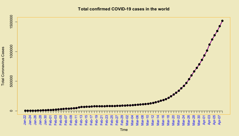
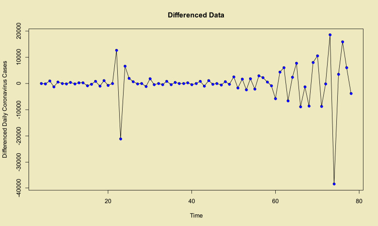
Time series plots of the total and daily cases in the world from 22-Jan up to 08-Apr of 2020 which are confirmed, and its stationary differenced with order 3 (i.e. ${\nabla }^3{X}_t=X_t-3X_{t-1}+3X_{t-2}+X_{t-3}$) are given in Fig. 1, Fig. 2 , respectively. Using the Dickey–Fuller test leads to p–value=0.01 with alternative hypothesis: stationary.

Fig. 1.

Time series plot of the total confirmed cases of COVID-19 in the world from 22-Jan up to 08-Apr of 2020.

Fig. 2.

Stationary time series plot of the COVID-19 in the world (differenced with order three).

Obviously number of cases (total and daily) in any days depend the number on them in the previous day(s), so the ARMA model can be suitable model for the COVID-19 cases data.

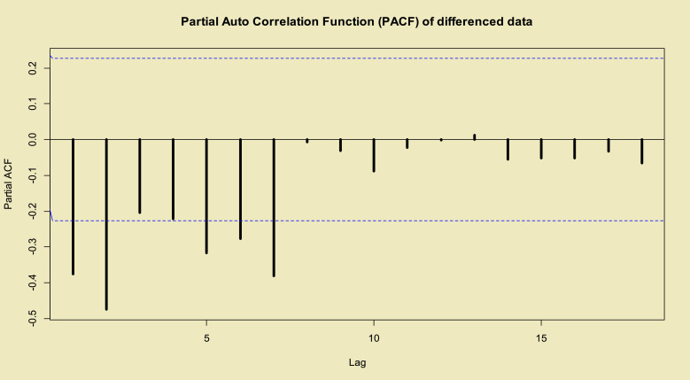
Two famous model selection criteria are Akaike information criteria ($AIC=2k-2l\left(\widehat{\Theta }\right)$; ref. [45]) and Bayesian information criteria ($BIC=k\log n-2l\left(\widehat{\Theta }\right)$; ref. [46]), k is the number of parameters that are estimated in fitted model. The proposed criteria have used to choose the best TP–SMN–ARMA model with the best fitted orders. These criteria and partial auto-correlation function (PACF) in Fig. 3 , demonstrate the following $TP--T--ARMA\left(7,0\right)$ is the best model

$$X_t+0.8994X_{t-1}+0.9817X_{t-2}+0.9336X_{t-3}+0.7858X_{t-4}+0.6506X_{t-5}+0.4597X_{t-6}+0.2662X_{t-7}=Z_t,$$

where

$$\left\{Z_t\right\}\sim \text{<italic>TP-T</italic>}\left(\mu =8.847374,\sigma =2766.178,\gamma =0.5362869,\nu =2.100046\right).$$

Fig. 3.

PACF of the stationary transformed total COVID-19 data in the world.

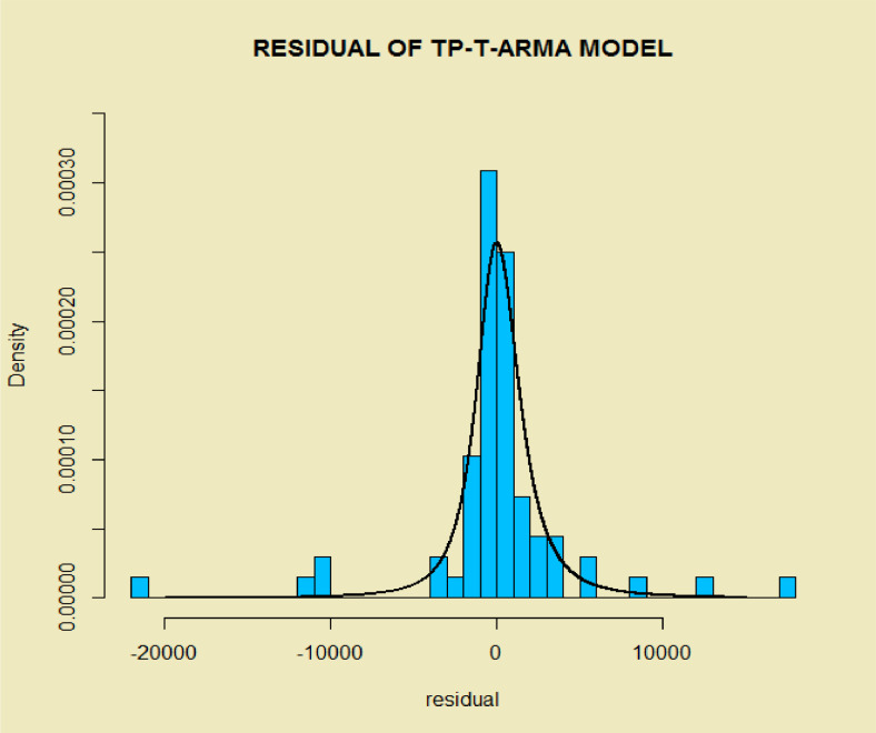
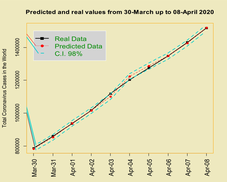
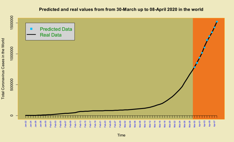
The histogram of the estimated errors (residuals) based on the estimated TP–T density (near symmetry but heavy-tailed) is superimposed on it shows the suitable performance of the estimated model to COVID-19 data (Fig. 4 ). To further demonstrate the good fit of the model, we eliminated the last 10 data (2020-Mar-30 up to 2020-Apr-08), then fitted the TP–SMN–ARMA model and forecast these data. Fig. 5, Fig. 6 and Table 1 , show the forecasted real values of the COVID-19 in the world data are close. Table 1 contains the predictions and 98% confidence intervals for them.

Fig. 4.

Histogram of the residuals of the fitted time series model on COVID-19 data in the world with superimposed estimated TP–T density.

Fig. 5.

Time series plot of real values and predicted COVID-19 data from 2020-Mar-30 up to 2020-Apr-08 with 98%.

Fig. 6.

Time series plot of COVID-19 data and predicted data from 2020-Mar-30 up to 08-Apr of 2020.

Table 1.

The real values of the COVID-19 in the world data from 2020-Mar-30 up to 2020-Apr-08 with predictions and 98% confidence interval.

Date	Real value	Prediction	Lower	Upper
2020-Mar-30	785,828	783,114	776,624	789,937
2020-Mar-31	859,620	852,651	845,272	859,197
2020-Apr-01	936,637	937,797	930,885	944,428
2020-Apr-02	1,016,734	1,016,045	1,008,173	1,022,633
2020-Apr-03	1,118,414	1,101,645	1,093,850	1,108,143
2020-Apr-04	1,203,235	1,223,923	1,215,528	1,230,375
2020-Apr-05	1,274,653	1,286,735	1,277,745	1,295,487
2020-Apr-06	1,348,564	1,348,163	1,338,874	1,357,682
2020-Apr-07	1,430,981	1,426,889	1,417,614	1,435,226
2020-Apr-08	1,518,023	1,520,874	1,511,512	1,529,308

The mean relative percentage error (MAPE) index given by

$$MAPE=\frac{1}{n}\sum _{i=1}^n\left|\frac{{\widehat{X}}_i-X_i}{X_i}\right|,$$

where ${\widehat{X}}_{n+1}=E\left(X_{n+1}{X}_n,\dots ,X_1\right),$ is then used to evaluate the accuracy of the suggested data prediction, which for the proposed predictions is 0.60% which shows the suitability of the proposed model for predicting. Note that, this criterion for the modeling via the ordinary Gaussian–ARMA model (also, the simplest TP–SMN–ARMA member) is 0.89%. Also the AIC and BIC criteria for the best fitted TP–SMN–ARMA are 1290.49 and 1298.02, and for the best fitted Gaussian–ARMA model are 1524.14 and 1544.12, respectively.

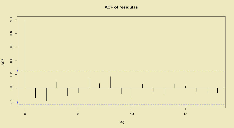
Finally, the p–value=0.972 from the Box–Pierce and p–value=0.931 from the Ljung–Box tests indicate the independency of residuals. Also the auto–correlation function (ACF) plot of the residuals presented in Fig. 7 shows the suitability of the $TP--T--ARMA\left(7,0\right)$ model to the total confirmed cased of the COVID-19 dataset.

Fig. 7.

ACF of the residuals of fitted time series model to total COVID-19 in the world data.

4.2. Death rate of COVID-19 data

In this section we consider and model the death rate of COVID-19 in the world from 02-Feb-2020 up to 08-Apr-2020, which this daily data also has reported by the China National Health Commission (NHC) and World Health Organization (WHO).

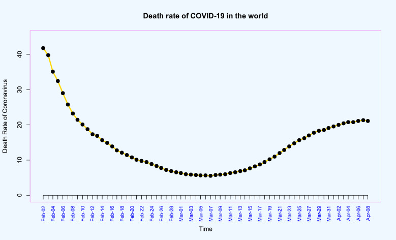
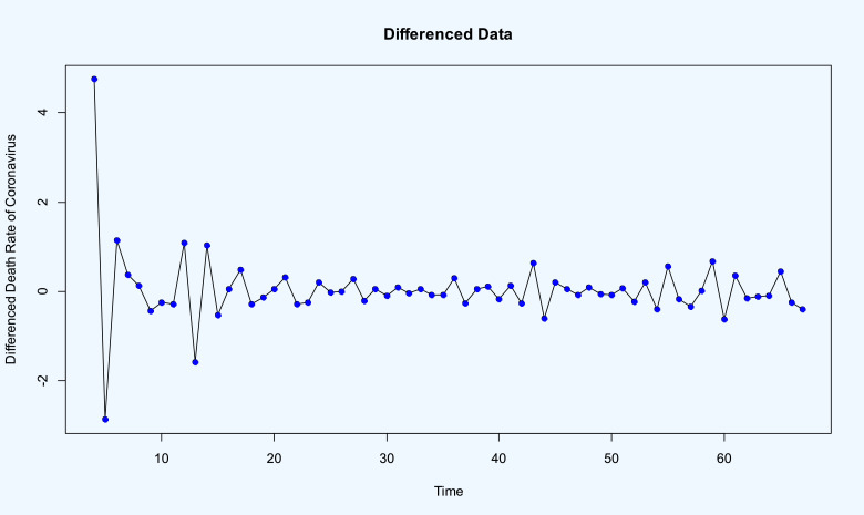
Time series plots of the death rate of coronavirus in the world from 02-Feb-2020 up to 08-Apr-2020, and its stationary differenced with order 3 (i.e. ${\nabla }^3{X}_t=X_t-3X_{t-1}+3X_{t-2}+X_{t-3}$) are given in Fig. 8, Fig. 9 , respectively. Using the Dickey–Fuller test leads to p–value=0.01 which demonstrate the stationarity of differenced data.

Fig. 8.

Time series plot of the death rate of COVID-19 in the world from 2020-Mar-30 up to 08-Apr of 2020.

Fig. 9.

Stationary time series plot of the death rate of COVID-19 in the world (differenced with order three).

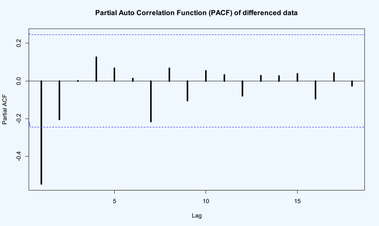
Using the model selection criteria and methodology in the previous data, demonstrate that best TP–SMN–ARMA model with the best fitted orders is $TP--T--ARMA\left(7,1\right)$. The PACF given in Fig. 10 also satisfies it. Therefore the following TP–SMN–ARMA is the best model

$$X_t+1.3760X_{t-1}+1.4183X_{t-2}+1.1401X_{t-3}+0.9269X_{t-4}+0.6482X_{t-5}+0.3181X_{t-6}+0.1752X_{t-7}=Z_t-.0628Z_{t-1},$$

where

$$\left\{Z_t\right\}\sim \text{<italic>TP-T</italic>}\left(\mu =0.056836,\sigma =0.2664454,\gamma =0.297544,\nu =2.826561\right).$$

Fig. 10.

PACF of the stationary transformed death rate of COVID-19 data in the world.

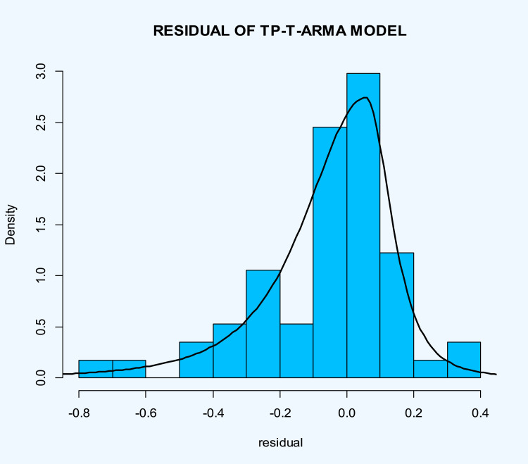
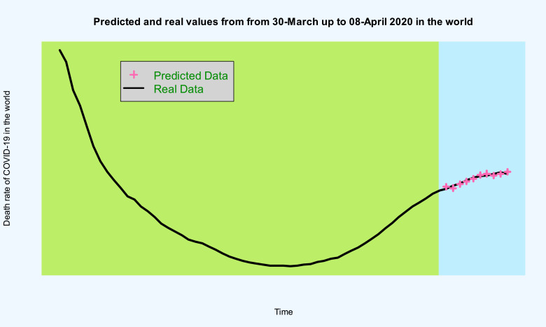
The histogram of the estimated errors (residuals) based on the estimated TP–T density (heavy-tailed and asymmetry) is superimposed on it shows the suitable performance of the estimated model to death rate of COVID-19 in the world (Fig. 11 ). Same as previous data, we eliminated the last 10 data (2020-Mar-30 up to 2020-Apr-08, then fitted the TP–SMN–ARMA model and forecast these data.

Fig. 11.

Histogram of the residuals of the fitted time series model on the death rate of COVID-19 in the world data with superimposed estimated TP–T density.

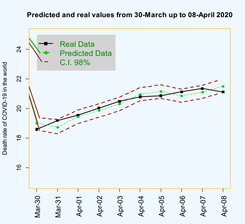
Figs. 12 , and 13 and Table 2 , show the forecasted real values of the death rate of COVID-19 in the world data are close. Table 2 contains the predictions and also 98% confidence intervals for them.

Fig. 12.

Time series plot of real values and predicted death rate of COVID-19 in the world data from 2020-Mar-30 up to 2020-Apr-28 with 98% confidence interval.

Fig. 13.

Time series plot of death rate of COVID-19 in the world data and predicted data from 2020-Mar-30 up to 2020-Mar-08.

Table 2.

The real values of the death rate of COVID-19 in the world data from 2020-Mar-30 up to 2020-Apr-08 with predictions and 98% confidence interval.

Date	Real value	Prediction	Lower	Upper
2020-Mar-30	18.59	19.00	18.55	19.39
2020-Mar-31	19.19	18.75	18.29	19.17
2020-Apr-01	19.55	19.45	18.98	19.89
2020-Apr-02	20.03	19.87	19.41	20.31
2020-Apr-03	20.48	20.32	19.86	20.76
2020-Apr-04	20.79	20.97	20.51	21.41
2020-Apr-05	20.86	21.16	20.70	21.60
2020-Apr-06	21.13	20.86	20.41	21.31
2020-Apr-07	21.35	21.12	20.68	21.59
2020-Apr-08	21.12	21.51	21.09	22.00

The MAPE for the second proposed predictions is 1.30% demonstrating the suitability of the proposed model for prediction. Note that, this criterion for the modeling via the ordinary Gaussian–ARMA model (also, the simplest TP–SMN–ARMA member) is 1.70%. Also the AIC and BIC criteria for the best fitted TP–SMN–ARMA are –4.42 and 18.05, and for the best fitted Gaussian–ARMA model are 76.68 and 95.07, respectively.

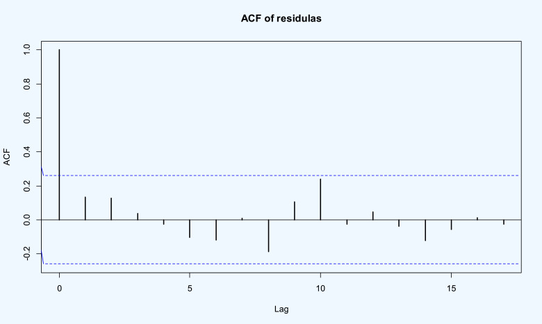
Finally, the p–value=0.974 from the Box–Pierce and p–value=0.873 from the Ljung–Box tests indicate the independence of residuals. Also, the ACF plot of the residuals presented in Fig. 14 demonstrates the suitability of the $TP-T-ARMA\left(7,1\right)$ model to the death rate of COVID-19 in the world dataset.

Fig. 14.

ACF of the residuals of the fitted time series model to the death rate of COVID-19 in the world data.

4. Conclusion

Coronaviruses are a huge family of viruses that affect neurological, gastrointestinal, hepatic, and respiratory systems. The numbers of confirmed cases are increased daily in different countries, especially in China, Iran, South Korea, Italy and others. The spread of the COVID-19 has many dangers and needs strict special plans and policies. Therefore, to consider the plans and policies, the predicting and forecasting the future confirmed cases are critical. The time series models are useful to model data that gathered and indexed by time. Classical time series is based on the symmetry of error's distribution. But there exist many situations in the real world that the assumption of symmetric distribution of the error terms is not satisfactory. In our methodology, we considered the time series models based on the two-piece scale mixture normal (TP–SMN) distributions. The proposed time series models were fitted initially to the historical COVID-19 datasets. Then, the time series that had the best fit to a dataset was selected. Finally, the selected models were applied to forecast the number of confirmed COVID-19 cases. The results indicate that the introduced approach acts well in forecasting the future confirmed COVID-19 cases. Also all of criteria demonstrate that the proposed models are more reasonable that the ordinary Gaussian time series model (, which also is the simplest members of our proposed model). Note that a sample copy of the code is available from the authors upon request.

Funding

No fund.

Declaration of Competing Interest

The authors declare no conflict of interest.

References

- 1.Chen Y., Liu Q., Guo D. Emerging coronaviruses: genome structure, replication, and pathogenesis. J Med Virol. 2020 doi: 10.1002/jmv.25681. [DOI] [PMC free article] [PubMed] [Google Scholar]
- 2.Ge X.Y., Li J.L., Yang X.L., Chmura A.A., Zhu G., Epstein J.H., Mazet J.K., Hu B., Zhang W., Peng C. Isolation and characterization of a bat SARS-like coronavirus that uses the ACE2 receptor. Nature. 2013;503:535–538. doi: 10.1038/nature12711. [DOI] [PMC free article] [PubMed] [Google Scholar]
- 3.Wang L.F., Shi Z., Zhang S., Field H., Daszak P., Eaton B.T. Review of bats and SARS. Emerg Infect Dis. 2006;12:1834. doi: 10.3201/eid1212.060401. [DOI] [PMC free article] [PubMed] [Google Scholar]
- 4.Cauchemez S., Van Kerkhove M., Riley S., Donnelly C., Fraser C., Ferguson N. Transmission scenarios for Middle East Respiratory Syndrome Coronavirus (MERS-CoV) and how to tell them apart. Euro Surveill Bull Eur Sur Les Mal Transm Eur Commun Dis Bull. 2013;18:20503. [PMC free article] [PubMed] [Google Scholar]
- 5.World Health Organization. Novel Coronavirus (2019-nCoV) 2020, 2020. Available online:https://www.who.int/ (accessed on 27 January 2020).
- 6.Lu R., Zhao X., Li J., Niu P., Yang B., Wu H., Wang W., Song H., Huang B., Zhu N.;. Genomic characterisation and epidemiology of 2019 novel coronavirus: implications for virus origins and receptor binding. Lancet. 2020;395:565–574. doi: 10.1016/S0140-6736(20)30251-8. [DOI] [PMC free article] [PubMed] [Google Scholar]
- 7.Cheng Z.J., Shan J. 2019 Novel Coronavirus: where We are and what we know. Infection. 2020 doi: 10.1007/s15010-020-01401-y. [DOI] [PMC free article] [PubMed] [Google Scholar]
- 8.Guan W.J., Ni Z.Y., Hu Y., Liang W.H., Ou C.Q., He J.X., Liu L., Shan H., Lei C.L., Hui D.S.;. Clinical characteristics of 2019 novel coronavirus infection in China. medRxiv. 2020 doi: 10.1101/2020.02.06.20020974. https://www.medrxiv.org/content/early/2020/02/09/2020.02.06.20020974.full.pdf Available online: (accessed on 9 February 2020) [DOI] [Google Scholar]
- 9.Zhao S., Musa S.S., Lin Q., Ran J., Yang G., Wang W., Lou Y., Yang L., Gao D., He D.;. Estimating the unreported number of Novel Coronavirus (2019-nCoV) cases in China in the first half of January 2020: a data-driven modelling analysis of the early outbreak. J Clin Med. 2020;9:388. doi: 10.3390/jcm9020388. [DOI] [PMC free article] [PubMed] [Google Scholar]
- 10.Nishiura H., Kobayashi T., Yang Y., Hayashi K., Miyama T., Kinoshita R., Linton N.M., Jung S.m., Yuan B., Suzuki A.;. The rate of underascertainment of Novel Coronavirus (2019-nCoV) infection: estimation using Japanese passengers data on evacuation flights. J Clin Med. 2020;9:419. doi: 10.3390/jcm9020419. [DOI] [PMC free article] [PubMed] [Google Scholar]
- 11.Tang B., Wang X., Li Q., Bragazzi N.L., Tang S., Xiao Y., Wu J. Estimation of the transmission risk of the 2019-nCoV and its implication for public health interventions. J Clin Med. 2020;9:462. doi: 10.3390/jcm9020462. [DOI] [PMC free article] [PubMed] [Google Scholar]
- 12.Thompson R.N. Novel Coronavirus outbreak in Wuhan, China, 2020: intense surveillance is vital for preventing sustained transmission in new locations. J Clin Med. 2020;9:498. doi: 10.3390/jcm9020498. [DOI] [PMC free article] [PubMed] [Google Scholar]
- 13.Jung S.M., Akhmetzhanov A.R., Hayashi K., Linton N.M., Yang Y., Yuan B. Real time estimation of the risk of death from novel coronavirus (2019-nCoV) infection: inference using exported cases. J Clin Med. 2020;9:523. doi: 10.3390/jcm9020523. [DOI] [PMC free article] [PubMed] [Google Scholar]
- 14.Al-qaness M.A.A., Ewees A.A., Fan H., Abd El Aziz M. Optimization method for forecasting confirmed cases of COVID-19 in China. J Clin Med. 2020;9:674. doi: 10.3390/jcm9030674. [DOI] [PMC free article] [PubMed] [Google Scholar]
- 15.DeFelice N.B., Little E., Campbell S.R., Shaman J. Ensemble forecast of human West Nile virus cases and mosquito infection rates. Nat Commun. 2017;8:1–6. doi: 10.1038/ncomms14592. [DOI] [PMC free article] [PubMed] [Google Scholar]
- 16.Ture M., Kurt I. Comparison of four different time series methods to forecast hepatitis A virus infection. Expert Syst Appl. 2006;31:41–46. [Google Scholar]
- 17.Shaman J., Karspeck A. Forecasting seasonal outbreaks of influenza. Proc Natl Acad Sci USA. 2012;109:20425–20430. doi: 10.1073/pnas.1208772109. J. Clin. Med. 2020, 9, 674 14 of 15. [DOI] [PMC free article] [PubMed] [Google Scholar]
- 18.Shaman J., Karspeck A., Yang W., Tamerius J., Lipsitch M. Real-time influenza forecasts during the 2012–2013 season. Nat Commun. 2013;4:1–10. doi: 10.1038/ncomms3837. [DOI] [PMC free article] [PubMed] [Google Scholar]
- 19.Shaman J., Yang W., Kandula S. Inference and forecast of the current West African Ebola outbreak in Guinea, Sierra Leone and Liberia. PLoS Curr. 2014:6. doi: 10.1371/currents.outbreaks.3408774290b1a0f2dd7cae877c8b8ff6. [DOI] [PMC free article] [PubMed] [Google Scholar]
- 20.Massad E., Burattini M.N., Lopez L.F., Coutinho F.A. Forecasting versus projection models in epidemiology: the case of the SARS epidemics. Med Hypotheses. 2005;65:17–22. doi: 10.1016/j.mehy.2004.09.029. [DOI] [PMC free article] [PubMed] [Google Scholar]
- 21.Ong J.B.S., Mark I., Chen C., Cook A.R., Lee H.C., Lee V.J. Real-time epidemic monitoring and forecasting of H1N1-2009 using influenza-like illness from general practice and family doctor clinics in Singapore. PLoS ONE. 2010;5 doi: 10.1371/journal.pone.0010036. [DOI] [PMC free article] [PubMed] [Google Scholar]
- 22.Nah K., Otsuki S., Chowell G., Nishiura H. Predicting the international spread of Middle East respiratory syndrome (MERS) BMC Infect Dis. 2016;16:356. doi: 10.1186/s12879-016-1675-z. [DOI] [PMC free article] [PubMed] [Google Scholar]
- 23.Mahmoudi M.R., Maleki M., Pak A. Testing the difference between two independent time series models. Iran J Sci Technol A (Sciences) 2017;41:665–669. [Google Scholar]
- 24.Mahmoudi M.R., Maleki M. A new method to detect periodically correlated structure. Comput Stat. 2017;32:1569–1581. [Google Scholar]
- 25.Maleki M., Arellano-Valle R.B. Maximum a-posteriori estimation of autoregressive processes based on finite mixtures of scale-mixtures of skew-normal distributions. J Stat Comput Sim. 2017;87:1061–1083. [Google Scholar]
- 26.Maleki M., Nematollahi A.R. Autoregressive models with mixture of scale mixtures of Gaussian innovations. Iran J Sci Technol A (Sciences) 2017;41:1099–1107. [Google Scholar]
- 27.Zarrin P., Maleki M., Khodadadi Z., Arellano-Valle R.B. Time series process based on the unrestricted skew normal process. J Stat Comput Sim. 2018;89:38–51. [Google Scholar]
- 28.Maleki M., Arellano-Valle R.B., Dey D.K., Mahmoudi M.R., Jalali S.M. A Bayesian approach to robust skewed Autoregressive process. Calcutta Statistical Association Bulltaine. 2018;69:165–182. [Google Scholar]
- 29.Hajrajabi A., Maleki M. Nonlinear semiparametric autoregressive model with finite mixtures of scale mixtures of skew normal innovations. J APPL STAT. 2019;46:2010–2029. [Google Scholar]
- 30.Maleki M., Wraith D., Mahmoudi M.R., Contreras-Reyes J.E. Asymmetric heavy-tailed vector auto-regressive processes with application to financial data. J Stat Comput Sim. 2020;90:324–340. [Google Scholar]
- 31.Ghasami S., Khodadadi Z., Maleki M. Autoregressive processes with generalized hyperbolic innovations. Commun Stat Simul Comput. 2018 doi: 10.1080/03610918.2018.1535066. [DOI] [Google Scholar]
- 32.Ghasami S., Maleki M., Khodadadi Z. Leptokurtic and Platykurtic class of robust symmetrical and asymmetrical time series models. J Comput Appl Math. 2020 doi: 10.1016/j.cam.2020.112806. [DOI] [Google Scholar]
- 33.Arellano-Valle R.B., Gómez H., Quintana F.A. Statistical inference for a general class of asymmetric distributions. J Stat Plan Infer. 2005;128:427–443. [Google Scholar]
- 34.Maleki M., Mahmoudi M.R. Two-piece location-scale distributions based on scale mixtures of normal family. Commun Stat Theory Methods. 2017;46:12356–12369. [Google Scholar]
- 35.Moravveji M., Khodadadi Z., Maleki M. A bayesian analysis of two-piece distributions based on the scale mixtures of normal family. Iran J Sci Technol A (Sciences) 2019;43:991–1001. [Google Scholar]
- 36.Maleki M., Mahmoudi M.R., Contreras-Reyes J.E. Robust mixture modeling based on two-piece scale mixtures of normal family. Axioms. 2019;8(2):38. [Google Scholar]
- 37.Maleki M., Barkhordar Z., Khodadadi Z., Wraith D. A robust class of homoscedastic nonlinear regression models. J Stat Comput Sim. 2019;89:2765–2781. doi: 10.1080/02664763.2020.1854203. [DOI] [PMC free article] [PubMed] [Google Scholar]
- 38.Hoseinzaseh A., Maleki M., Khodadadi Z., Contreras-Reyes J.E. The Skew-Reflected-Gompertz distribution for analyzing symmetric and asymmetric data. J Comput Appl Math. 2019;349:132–141. [Google Scholar]
- 39.Whittle P. Almquist and Wicksell; 1951. Hypothesis Testing in Time Series Analysis. [Google Scholar]
- 40.Box George, Jenkins Gwilym M, Reinsel Gregory C. 3rd ed. Prentice-Hall; 1994. Time series analysis: forecasting and control. ISBN 0130607746. [Google Scholar]
- 41.Brockwell P.J., Davis R.A. 2nd ed. Springer; New York: 2009. Time series: theory and methods. [Google Scholar]
- 42.Brockwell P.J., Davis R.A. 2nd ed. Springer Science & Business Media; 2002. Introduction to time series and forecasting (Springer texts in statistics) [Google Scholar]
- 43.Andrews D.R., Mallows C.L. Scale mixture of normal distribution. J R Stat Soc B. 1974;36:99–102. [Google Scholar]
- 44.Dempster A.P., Laird N.M., Rubin D.B. Maximum likelihood from incomplete data via the EM algorithm. J R Stat Soc B. 1977;39:1–22. [Google Scholar]
- 45.Akaike H. A new look at the statistical model identification. IEEE T Automa Contr. 1974;19:716–723. [Google Scholar]
- 46.Schwarz G. Estimating the dimension of a model. Ann Stat. 1978;6:461–464. [Google Scholar]