Figure 5.

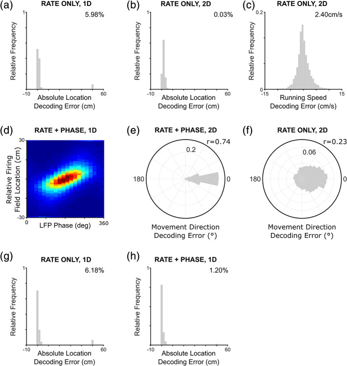
Decoding movement trajectories from grid cell population activity in each oscillatory cycle. Location in both (a) one‐dimensional (1D) and (b) two‐dimensional (2D) environments can be decoded from population firing rates, using the grid cell rate function (frequency of catastrophic errors inset). (c) In addition, running speed can be decoded from the total number of spikes fired by the grid cell population (standard deviation inset). (d) Phase precession across the grid cell population generates “theta sequences” of activity within each oscillatory cycle that correspond to the current movement trajectory (color axis indicates spike density). (e) This allows movement direction to be estimated from the sequence of locations decoded across phase bins (resultant vector length inset). (f) Conversely, in the absence of a phase code for location, movement direction decoding is much less accurate (resultant vector length inset). (g) Location can also be decoded from population firing rates, using the history of firing rates across oscillatory cycles in that simulation (frequency of catastrophic errors inset). (h) However, decoding location using both population firing rate and phase information is more accurate, as illustrated by a significant reduction in the rate of catastrophic errors (frequency of catastrophic errors inset). Panels a, b, g, and h are averaged over data from 20 independent simulations [Color figure can be viewed at wileyonlinelibrary.com]