On the dynamical modeling of COVID-19 involving Atangana–Baleanu fractional derivative and based on Daubechies framelet simulations

Abstract

In this paper, we present a novel fractional order COVID-19 mathematical model by involving fractional order with specific parameters. The new fractional model is based on the well-known Atangana–Baleanu fractional derivative with non-singular kernel. The proposed system is developed using eight fractional-order nonlinear differential equations. The Daubechies framelet system of the model is used to simulate the nonlinear differential equations presented in this paper. The framelet system is generated based on the quasi-affine setting. In order to validate the numerical scheme, we provide numerical simulations of all variables given in the model.

1. Introduction

The novel corona-virus is a new strain of coronavirus which may cause illness, fever, dry cough where these symptoms are usually mild and begin gradually. The world health organization has declared this virus as a pandemic in early March of 2020 where many countries have taken serious actions and implemented curfew, quarantine and lock-down measures as a plan to control the rapid spread of COVID-19. The first case of COVID-19 was detected in Wuhan city in China at the end of the year of 2019 where it is suggested that the COVID-19 virus might be originated from bats and it’s transmission might related to a seafood market exposure. Many researchers worldwide started to work on developing mathematical models that best describe the dynamics of this pandemic. It is known in biological system with memory it would be suitable to use fractional derivatives to describe evolution of the system [1], [2], [3], [4], [5], [6], [7], [8], [9], [10]. Furthermore, Atangana–Baleanu fractional derivative (ABFD) has been one of the most useful operators for modeling non-local behaviors by fractional differential equations. The advantage of using such derivative lies on its properties such as the non-locality and non-singularity of its kernel, and the crossover behavior in the model can only be best described using this derivative. Additionally, it allows traditional and various types of initial conditions to be consider in the creation of the dynamical model. Many scientists proposed new models to best describe the dynamics of all possible parameters responsible for the daily cases reported including deaths, control the fatality rate, and prediction of COVID-19 behavior in future within a specific region. It is known that several models can describe the same system, which is a challenging step. In this paper we intend to formulate a new mathematical model of Corona virus based on the model presented in Ndaïrou et al. [11] based on ABFD. The numerical method simulation is conducted via the framelet system generated using Daubechies scaling functions.

Daubechies wavelets have been proven as a useful tool in a variety of various applications such as filter banks constructions in image painting. This is largely due to the fact that wavelets have the right structure to capture the sparsity in âphysicalâ images, perfect mathematical properties such as its multi-scale structure, sparsity, smoothness, compactly supported, and high vanishing moments properties. It has many applications in fractional integral and differential equations (see for example [12], [13], [14], [15], [16], [17], [18], [19], [20], [21], [22], [23], [24], [25], [26], [27], [28]. Framelets have been used extensively in the context of both pure and numerical methods in several applications, due to their well prevailing and recognized theory and its natural properties such as sparsity and stability which lead to a well-conditioned scheme. In this paper, an effective and accurate technique based on Daubechies wavelets is presented for solving the transmission model of COVID-19 based on Caputo fractional derivative. The advantage of using such wavelets, lies on its simple structure of the reduced systems and in the powerfulness of obtaining approximated solutions for such equations that have weakly singular kernels. The proposed method shows a good performance and high accuracy orders.

Definition 1.1

A function $\varphi \in L_2\left(\mathbb{R}\right)$ is called a scaling function if

$$\varphi =2\sum _{k\mathbb{Z}}a\left[k\right]\varphi (2·-k),$$ (1.1)

where $a\left[k\right]\in {\ell }_2\left(\mathbb{Z}\right)$ is finitely supported sequence and is called the refinement mask of ϕ. The corresponding wavelet function is defined by

$$\psi =2\sum _{k\mathbb{Z}}b\left[k\right]\varphi (2·-k),$$ (1.2)

where $b\left[k\right]\in {\ell }_2\left(\mathbb{Z}\right)$ is finitely supported sequence and is called the high pass filter of ψ.

For a function $f\in L_1\left(\mathbb{R}\right)$ (which can be naturaly extended to $L_2\left(\mathbb{R}\right)$), we use the following Fourier transform defined by

$$\widehat{f}\left(\xi \right)=\frac{1}{\sqrt{2\pi }}{\int }_{\mathbb{R}}{e}^{-ix\xi }f\left(x\right)dx.$$

The Fourier series of the sequence a is defined by

$$\widehat{a}\left(\xi \right)=\sum _{k\in \mathbb{Z}}a\left[k\right]e^{-ik\xi },\xi \in \mathbb{R}.$$ (1.3)

2. Daubechies framelets using the unitary extension principle (UEP)

If g is a wavelet function that has q vanishing moments such that

$$\int t^{m}g\left(t\right)dt=0,m=0,1,\dots ,q-1.$$

Suppose that the function g generates an orthonormal basis of $L^2\left(\mathbb{R}\right),$ then the constructed wavelet will be compactly supported within the domain $[0,2q-1].$ Daubechies wavelets do not have explicit form but defined recursively as follows

$$\begin{array}{ccc}\hfill g_m\left(x\right)& =& \sqrt{2}\sum _{k\in \mathbb{Z}}{h}_k{\varphi }_{m-1}(2x-k),\hfill \\ \hfill g_0\left(x\right)& =& {\chi }_{[0,1)}\left(x\right).\hfill \end{array}$$

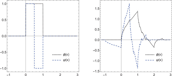
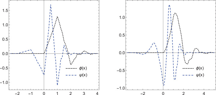
One of the important features of this wavelet is its smoothness as it increases for a higher q. We present the graphs of ϕ and its corresponding wavelet ψ when $q=1,2$ and 3,4 in Figs. 1 and 2 respectively.

Definition 2.1

A sequence ${\left\{g_k\right\}}_{k=1}^{\infty }$ of functions in $L^2\left(\mathbb{R}\right)$ is called a frame for $L^2\left(\mathbb{R}\right)$ if ∃ postive numbers r, R such that

$${r\parallel f\parallel }^2\le \sum _{k=1}^{\infty }{\left|〈g,g_k〉\right|}^2\le R{\parallel f\parallel }^2\text{,}\forall g\in L^2\left(\mathbb{R}\right).$$

The constants r, R are called frame bounds [29]. A frame is called tight if we have $r=R$ as frame bounds, and it is Parseval frame if $r=R=1.$

Fig. 1.

Daubechies refinable functions with their corresponding wavelets of order $q=1$ and $q=2$ respectively.

Fig. 2.

Daubechies refinable functions with their corresponding wavelets of order $q=3$ and $q=4$ respectively.

The idea is to construct framelet system based on Daubechies scaling function ϕ and its corresponding wavelet function ψ. Assume that $\Xi ={\left\{{\psi }_{\ell }\right\}}_{\ell =1}^r\subset L^2\left(\mathbb{R}\right)$ such that

$${\psi }_{\ell }=2\sum _{k\in \mathbb{Z}}{b}_{\ell }\left[k\right]\varphi (2·-k),$$ (2.1)

where ${\{b_{\ell }\left[k\right]\text{,}k\in \mathbb{Z}\}}_{\ell =1}^r$ is a finitely supported sequence. Define the wavelet system

$$X\left(\Xi \right)=\{{\psi }_{\ell ,j,k}:1\le \ell \le r;j,k\in \mathbb{Z}\},$$

where ${\psi }_{\ell ,j,k}\left(x\right)=2^{j/2}{\psi }_{\ell }(2^{j}x-k)$.

Theorem 2.2 UEP [29] —

Assume that $\varphi \in L^2\left(\mathbb{R}\right)$ be a compactly supported scaling function. Let ${\{b_{\ell }\left[k\right],k\in \mathbb{Z}\}}_{\ell =1}^r$ be a set of finitely supported sequences, then

$$X\left(\Xi \right)=\{{\psi }_{\ell ,j,k}:1\le \ell \le r;j,k\in \mathbb{Z}\}$$ (2.2)

generates a framelet system for $L^2\left(\mathbb{R}\right)$ if the following is hold for any $d\in \mathbb{Z}$

$$\sum _{\ell =0}^r\sum _{k\in \mathbb{Z}}\overline{b_{\ell }\left[k\right]}{b}_{\ell }[k-p]={\delta }_{0,d}$$ (2.3)

and

$$\sum _{\ell =0}^r\sum _{k\in \mathbb{Z}}{(-1)}^{k-d}\overline{b_{\ell }\left[k\right]}{b}_{\ell }[k-d]=0.$$ (2.4)

According to Theorem 2.2, for any constructed framelet system we have the following representation given by

$$f=\sum _{\ell =1}^r\sum _{j\in \mathbf{Z}}\sum _{k\in \mathbf{Z}}〈f,{\psi }_{\ell ,j,k}〉{\psi }_{\ell ,j,k}.$$ (2.5)

This system can be truncated by ${\mathcal{U}}_{n}f$ as follows

$${\mathcal{U}}_{n}f=\sum _{\ell =1}^r\sum _{j<n}\sum _{k\in \mathbf{Z}}〈f,{\psi }_{\ell ,j,k}〉{\psi }_{\ell ,j,k}.$$ (2.6)

2.1. Examples of Daubechies framelet systems

Here we provide some examples on the construction of framelet systems basd on several orders of Daubechies scaling functions of different orders.

Example 2.1

For $q=1,$ let $a\left[k\right]=[0.5,0.5]$. Then based on the UEP, we can find two finitely supported sequences b ₁[k], b ₂[k] such that the following two functions generate a framelet system of $L^2\left(\mathbb{R}\right)$

$$\begin{array}{ccc}\hfill {\widehat{\psi }}_1\left(\xi \right)& =& -\frac{\left(0.282238i\right)e^{\left(0.5i\right)\xi }}{\xi }+\frac{0.282238i}{\xi }-\frac{0.564477e^{\left(0.75i\right)\xi }\sin \left(0.25\xi \right)}{\xi },\hfill \\ \hfill {\widehat{\psi }}_2\left(\xi \right)& =& \frac{\left(0.282238i\right)e^{\left(0.5i\right)\xi }}{\xi }-\frac{0.282238i}{\xi }+\frac{0.564477e^{\left(0.75i\right)\xi }\sin \left(0.25\xi \right)}{\xi }.\hfill \end{array}$$

Note that, according to the UEP we need to solve the following system of equation written in MATLAB software to be able to get the required sequences b ₁[k], b ₂[k], where for $q=1$ we have

$$\begin{array}{ccc}\hfill functionF& =& mydaub2\left(x\right)\hfill \\ \hfill F& =& [{\left(x\left(1\right)\right)}^2+{\left(x\left(2\right)\right)}^2+{\left(x\left(3\right)\right)}^2+{\left(x\left(4\right)\right)}^2-.5;x\left(1\right)*x\left(2\right)+x\left(3\right)*x\left(4\right)+(1/4);\hfill \\ & & {\left(x\left(1\right)\right)}^2-{\left(x\left(2\right)\right)}^2+{\left(x\left(3\right)\right)}^2-{\left(x\left(4\right)\right)}^2];\hfill \\ & & end;\hfill \end{array}$$

and for $q=2$ we have the following

$$\begin{array}{ccc}\hfill functionF& =& mydaub4\left(x\right)\hfill \\ \hfill F& =& [{\left(x\left(1\right)\right)}^2+{\left(x\left(2\right)\right)}^2+{\left(x\left(3\right)\right)}^2+{\left(x\left(4\right)\right)}^2+{\left(x\left(5\right)\right)}^2+{\left(x\left(6\right)\right)}^2+{\left(x\left(7\right)\right)}^2+{\left(x\left(8\right)\right)}^2-(1/2);\hfill \\ & & x\left(1\right)*x\left(2\right)+x\left(2\right)*x\left(3\right)+x\left(3\right)*x\left(4\right)+x\left(5\right)*x\left(6\right)+x\left(6\right)*x\left(7\right)+x\left(7\right)*x\left(8\right)+(9/32);\hfill \\ & & x\left(1\right)*x\left(3\right)+x\left(2\right)*x\left(4\right)+x\left(5\right)*x\left(7\right)+x\left(6\right)*x\left(8\right);\hfill \\ & & x\left(1\right)*x\left(4\right)+x\left(5\right)*x\left(8\right)+(-1/32);\hfill \\ & & {\left(x\left(1\right)\right)}^2-{\left(x\left(2\right)\right)}^2+{\left(x\left(3\right)\right)}^2-{\left(x\left(4\right)\right)}^2+{\left(x\left(5\right)\right)}^2-{\left(x\left(6\right)\right)}^2+{\left(x\left(7\right)\right)}^2-{\left(x\left(8\right)\right)}^2+(-585/2702);\hfill \\ & & x\left(1\right)*x\left(2\right)-x\left(2\right)*x\left(3\right)+x\left(3\right)*x\left(4\right)+x\left(5\right)*x\left(6\right)-x\left(6\right)*x\left(7\right)+x\left(7\right)*x\left(8\right)+(3/32);\hfill \\ & & x\left(1\right)*x\left(3\right)-x\left(2\right)*x\left(4\right)+x\left(5\right)*x\left(7\right)-x\left(6\right)*x\left(8\right)+(484/4471)];\hfill \\ & & end;\hfill \end{array}$$

where x(k) is the nonzero value of the compactly supported sequences of both b ₁ and b ₂. Note that, when $q=2,$ we have the following low pass filter

$$a\left[k\right]=[\frac{1+\sqrt{3}}{8},\frac{3+\sqrt{3}}{8},\frac{3-\sqrt{3}}{8},\frac{1-\sqrt{3}}{8}]$$

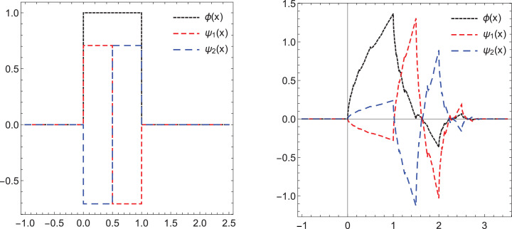
The graphs of Daubechies scaling functions of order one and two along with their corresponding framelets are depicted in Fig. 3 .

Example 2.2

For $q=3,$ we have the following low pass filter related to Daubechies scaling function of order 3 given by

$$a\left[k\right]=[0.235233,0.5705584,0.325182,-0.095467,-0.06041610,0.0249087].$$

Then based on the UEP, we can find two finitely supported sequences b ₁[k], b ₂[k] such that two functions ψ ₁, ψ ₂ can generate a framelet system of $L^2\left(\mathbb{R}\right)$. Note that, according to the UEP we need to solve the following system of equation written in MATLAB software to be able to get the required sequences b ₁[k], b ₂[k], where for $q=3$ we have

$$\begin{array}{ccc}\hfill functionF& =& mydaub6\left(x\right)\hfill \\ \hfill F& =& [{\left(x\left(1\right)\right)}^2+{\left(x\left(2\right)\right)}^2+{\left(x\left(3\right)\right)}^2+{\left(x\left(4\right)\right)}^2+{\left(x\left(5\right)\right)}^2+{\left(x\left(6\right)\right)}^2+{\left(x\left(7\right)\right)}^2+{\left(x\left(8\right)\right)}^2+{\left(x\left(9\right)\right)}^2+\hfill \\ & & {\left(x\left(10\right)\right)}^2+{\left(x\left(11\right)\right)}^2+{\left(x\left(12\right)\right)}^2-.5;\hfill \\ & & x\left(1\right)*x\left(2\right)+x\left(2\right)*x\left(3\right)+x\left(3\right)*x\left(4\right)+x\left(4\right)*x\left(5\right)+x\left(5\right)*x\left(6\right)+x\left(7\right)*x\left(8\right)+\hfill \\ & & x\left(8\right)*x\left(9\right)+x\left(9\right)*x\left(10\right)+x\left(10\right)*x\left(11\right)+x\left(11\right)*x\left(12\right)+(75/256);\hfill \\ & & x\left(1\right)*x\left(3\right)+x\left(2\right)*x\left(4\right)+x\left(3\right)*x\left(5\right)+x\left(4\right)*x\left(6\right)+x\left(7\right)*x\left(9\right)+\hfill \\ & & x\left(10\right)*x\left(8\right)+x\left(11\right)*x\left(9\right)+x\left(12\right)*x\left(10\right)+\left(0\right);\hfill \\ & & x\left(1\right)*x\left(4\right)+x\left(2\right)*x\left(5\right)+x\left(6\right)*x\left(3\right)+x\left(10\right)*x\left(7\right)+x\left(11\right)*x\left(8\right)+\hfill \\ & & x\left(12\right)*x\left(9\right)+(-25/512);x\left(1\right)*x\left(5\right)+x\left(2\right)*x\left(6\right)+x\left(11\right)*x\left(7\right)+\hfill \\ & & x\left(12\right)*x\left(8\right)+\left(0\right);x\left(1\right)*x\left(6\right)+x\left(12\right)*x\left(7\right)+(3/512);\hfill \\ & & {\left(x\left(1\right)\right)}^2-{\left(x\left(2\right)\right)}^2+{\left(x\left(3\right)\right)}^2-{\left(x\left(4\right)\right)}^2+{\left(x\left(5\right)\right)}^2-{\left(x\left(6\right)\right)}^2+\hfill \\ & & {\left(x\left(7\right)\right)}^2-{\left(x\left(8\right)\right)}^2+{\left(x\left(9\right)\right)}^2-{\left(x\left(10\right)\right)}^2+{\left(x\left(11\right)\right)}^2-{\left(x\left(12\right)\right)}^2+(-22/129);\hfill \\ & & x\left(1\right)*x\left(2\right)-x\left(2\right)*x\left(3\right)+x\left(3\right)*x\left(4\right)-x\left(4\right)*x\left(5\right)+x\left(5\right)*x\left(6\right)+x\left(7\right)*x\left(8\right)-\hfill \\ & & x\left(8\right)*x\left(9\right)+x\left(9\right)*x\left(10\right)-x\left(10\right)*x\left(11\right)+x\left(11\right)*x\left(12\right)+(-468/5221);\hfill \\ & & x\left(1\right)*x\left(3\right)-x\left(2\right)*x\left(4\right)+x\left(3\right)*x\left(5\right)-x\left(4\right)*x\left(6\right)+x\left(7\right)*x\left(9\right)-x\left(10\right)*x\left(8\right)+\hfill \\ & & x\left(11\right)*x\left(9\right)-x\left(12\right)*x\left(10\right)+(44/387);x\left(1\right)*x\left(4\right)-x\left(2\right)*x\left(5\right)+\hfill \\ & & x\left(3\right)*x\left(6\right)+x\left(10\right)*x\left(7\right)-x\left(11\right)*x\left(8\right)+x\left(12\right)*x\left(9\right)+(329/16357);\hfill \\ & & x\left(1\right)*x\left(5\right)-x\left(2\right)*x\left(6\right)+x\left(11\right)*x\left(7\right)-x\left(12\right)*x\left(8\right)+(-11/387);];\hfill \\ \hfill end;\end{array}$$

For $q=4,$ we have the following low pass filter

$$\begin{array}{ccc}\hfill a\left[k\right]& =& [0.1629017,0.50547285,0.4461000,-0.01978751,\hfill \\ & & -0.1322535,0.02180815,.0232518005,-0.00749349,\hfill \\ & & -0.1322535836,0.021808150,0.0232518005,-0.00749349]\hfill \end{array}$$

Again we need to solve a bigger system to obtain sequences b ₁[k], b ₂[k], where x(k) is the nonzero values of the supported sequences. The system is given by the following

$$\begin{array}{c}\hfill functionF=mydaub8\left(x\right)\\ \hfill F=[{\left(x\left(1\right)\right)}^2+{\left(x\left(2\right)\right)}^2+{\left(x\left(3\right)\right)}^2+{\left(x\left(4\right)\right)}^2+{\left(x\left(5\right)\right)}^2+{\left(x\left(6\right)\right)}^2+{\left(x\left(7\right)\right)}^2+\\ \hfill {\left(x\left(8\right)\right)}^2+{\left(x\left(9\right)\right)}^2+{\left(x\left(10\right)\right)}^2+{\left(x\left(11\right)\right)}^2+{\left(x\left(12\right)\right)}^2+{\left(x\left(13\right)\right)}^2+{\left(x\left(14\right)\right)}^2+\\ \hfill {\left(x\left(15\right)\right)}^2+{\left(x\left(16\right)\right)}^2-(1/2);x\left(1\right)*x\left(2\right)+x\left(2\right)*x\left(3\right)+x\left(3\right)*x\left(4\right)+x\left(4\right)*x\left(5\right)+\\ \hfill x\left(5\right)*x\left(6\right)+x\left(6\right)*x\left(7\right)+x\left(7\right)*x\left(8\right)+x\left(9\right)*x\left(10\right)+x\left(10\right)*x\left(11\right)+x\left(11\right)*x\left(12\right)+\\ \hfill x\left(12\right)*x\left(13\right)+x\left(13\right)*x\left(14\right)+x\left(14\right)*x\left(15\right)+x\left(15\right)*x\left(16\right)+(419/1401);\\ \hfill x\left(1\right)*x\left(3\right)+x\left(2\right)*x\left(4\right)+x\left(3\right)*x\left(5\right)+x\left(4\right)*x\left(6\right)+x\left(5\right)*x\left(7\right)+x\left(6\right)*x\left(8\right)+\\ \hfill x\left(9\right)*x\left(11\right)+x\left(10\right)*x\left(12\right)+x\left(11\right)*x\left(13\right)+x\left(12\right)*x\left(14\right)+x\left(13\right)*x\left(15\right)+\\ \hfill x\left(14\right)*x\left(16\right)+;x\left(1\right)*x\left(4\right)+x\left(2\right)*x\left(5\right)+x\left(3\right)*x\left(6\right)+x\left(4\right)*x\left(7\right)+\\ \hfill x\left(5\right)*x\left(8\right)+x\left(9\right)*x\left(12\right)+x\left(10\right)*x\left(13\right)+x\left(11\right)*x\left(14\right)+x\left(12\right)*x\left(15\right)+\\ \hfill x\left(13\right)*x\left(16\right)+(-245/4096);x\left(1\right)*x\left(5\right)+x\left(2\right)*x\left(6\right)+x\left(3\right)*x\left(7\right)+x\left(4\right)*x\left(8\right)+\\ \hfill x\left(9\right)*x\left(13\right)+x\left(10\right)*x\left(14\right)+x\left(11\right)*x\left(15\right)+x\left(12\right)*x\left(16\right)+\left(0\right);\end{array}$$

$$\begin{array}{c}\hfill x\left(1\right)*x\left(6\right)+x\left(2\right)*x\left(7\right)+x\left(3\right)*x\left(8\right)+x\left(9\right)*x\left(14\right)+x\left(10\right)*x\left(15\right)+\\ \hfill x\left(11\right)*x\left(16\right)+(49/4096);x\left(1\right)*x\left(7\right)+x\left(2\right)*x\left(8\right)+x\left(9\right)*x\left(15\right)+\\ \hfill x\left(10\right)*x\left(16\right)+\left(0\right);x\left(1\right)*x\left(8\right)+x\left(9\right)*x\left(16\right)+(-5/4096);\\ \hfill {\left(x\left(1\right)\right)}^2-{\left(x\left(2\right)\right)}^2+{\left(x\left(3\right)\right)}^2-{\left(x\left(4\right)\right)}^2+{\left(x\left(5\right)\right)}^2-{\left(x\left(6\right)\right)}^2+\\ \hfill {\left(x\left(7\right)\right)}^2-{\left(x\left(8\right)\right)}^2+{\left(x\left(9\right)\right)}^2-{\left(x\left(10\right)\right)}^2+{\left(x\left(11\right)\right)}^2-{\left(x\left(12\right)\right)}^2+\\ \hfill {\left(x\left(13\right)\right)}^2-{\left(x\left(14\right)\right)}^2+{\left(x\left(15\right)\right)}^2-{\left(x\left(16\right)\right)}^2+(-26/2023);\\ \hfill x\left(1\right)*x\left(2\right)-x\left(2\right)*x\left(3\right)+x\left(3\right)*x\left(4\right)-x\left(4\right)*x\left(5\right)+x\left(5\right)*x\left(6\right)-x\left(6\right)*x\left(7\right)+\\ \hfill x\left(7\right)*x\left(8\right)+x\left(9\right)*x\left(10\right)-x\left(10\right)*x\left(11\right)+x\left(11\right)*x\left(12\right)-x\left(12\right)*x\left(13\right)+\\ \hfill x\left(13\right)*x\left(14\right)-x\left(14\right)*x\left(15\right)+x\left(15\right)*x\left(16\right)+(-536/3389);\\ \hfill x\left(1\right)*x\left(3\right)-x\left(2\right)*x\left(4\right)+x\left(3\right)*x\left(5\right)-x\left(4\right)*x\left(6\right)+x\left(5\right)*x\left(7\right)-x\left(6\right)*x\left(8\right)+\\ \hfill x\left(9\right)*x\left(11\right)-x\left(10\right)*x\left(12\right)+x\left(11\right)*x\left(13\right)-x\left(12\right)*x\left(14\right)+x\left(13\right)*x\left(15\right)+\\ \hfill -x\left(14\right)*x\left(16\right)+(202/9531);x\left(1\right)*x\left(4\right)-x\left(2\right)*x\left(5\right)+x\left(3\right)*x\left(6\right)-x\left(4\right)*x\left(7\right)+\\ \hfill x\left(5\right)*x\left(8\right)+x\left(9\right)*x\left(12\right)-x\left(10\right)*x\left(13\right)+x\left(11\right)*x\left(14\right)-x\left(12\right)*x\left(15\right)+\\ \hfill x\left(13\right)*x\left(16\right)+(155/2072);x\left(1\right)*x\left(5\right)-x\left(2\right)*x\left(6\right)+x\left(3\right)*x\left(7\right)+\\ \hfill -x\left(4\right)*x\left(8\right)+x\left(9\right)*x\left(13\right)-x\left(10\right)*x\left(14\right)+x\left(11\right)*x\left(15\right)-x\left(12\right)*x\left(16\right)+(-127/5684);\\ \hfill x\left(1\right)*x\left(6\right)-x\left(2\right)*x\left(7\right)+x\left(3\right)*x\left(8\right)+x\left(9\right)*x\left(14\right)-x\left(10\right)*x\left(15\right)+x\left(11\right)*x\left(16\right)+\\ \hfill (-224/19405);x\left(1\right)*x\left(7\right)-x\left(2\right)*x\left(8\right)+x\left(9\right)*x\left(15\right)-x\left(10\right)*x\left(16\right)+(238/31417)];\\ \hfill end;\end{array}$$

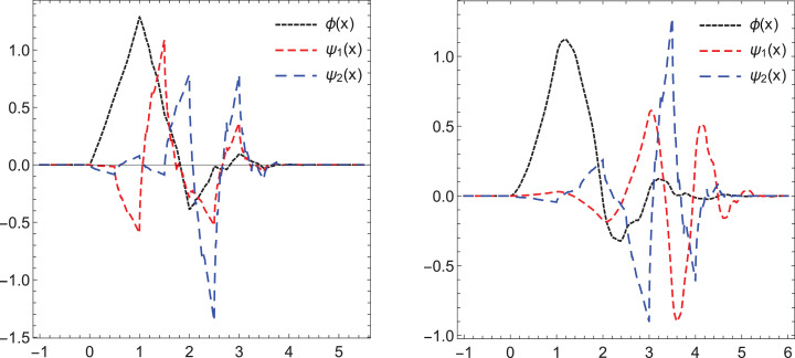
We present the graphs of Daubechies scaling functions of order three and four along with their corresponding framelets in Fig. 4 .

Fig. 3.

Daubechies framelet generators with their corresponding scaling functions for $q=1$ and $q=2$ respectively.

Fig. 4.

Daubechies framelet generators with their corresponding scaling functions for $q=3$ and $q=4$ respectively.

Given the construction in the first part above and to simulate the resulting equations, now we are ready to introduce the new COVID-19 fractional model of nonlinear differential equations by applying the Atangana–Baleanu derivative. The advantage of using such framelet lies in its properties such as the highest number of vanishing moments, redundancy and its applications in solving a broad range of problems such as fractal problems and function discontinuities, see e.g., [13].

3. ABFD of COVID-19 model

Herein, we consider the model presented in Ndaïrou et al. [11] using ABFD. The model has eight nonlinear DEs. To simulate the system and for simplicity, we consider Daubechies framelet system of order one.

Hence, the new modified model that obtained by changing the left hand side of the system presented in Ndaïrou et al. [11] by involving ABFD. Before presenting the new model in fractional sense, let us provide the definition of ABFD and its associated integral. The advantage of using such framelets lies

Definition 3.1

For a real function u(t) where t, α > 0 and $n\in \mathbb{N},$ we have the following fractional operators of order α, namely:

• •
  The ABFD sense,

  $${}_a^{ABC}{\mathcal{D}}_t^{\alpha }u\left(t\right)=\frac{\mathcal{B}\left(\alpha \right)}{1-\alpha }{\int }_a^t{u}^{\prime }\left(y\right)M_{\alpha }(-\frac{\alpha }{1-\alpha }{(t-y)}^{\alpha })dy,$$

  where $\mathcal{B}\left(\alpha \right)$ is a normalization function such that $\mathcal{B}\left(0\right)=\mathcal{B}\left(1\right)=0$ and M_α is the MittagâLeffler function.
• •
  The integral operator corresponding to this definition is given by

  $${\mathcal{I}}^{\alpha }u\left(x\right)=\frac{(1-\alpha )u\left(x\right)}{B\left(\alpha \right)}+\frac{\alpha }{B\left(\alpha \right)\Gamma \left(\alpha \right)}{\int }_0^x\frac{u\left(t\right)}{{(x-t)}^{1-\alpha }}dt.$$ (3.1)

We refer the reader to [4], [5] for more details and properties of the fractional derivative.

Therefore, the new model can be written as follows

$${}_a^{ABC}{\mathcal{D}}_t^{\alpha }S\left(t\right)=-\frac{\beta \iota H\left(t\right)S\left(t\right)}{N}-\frac{\beta P\left(t\right)S\left(t\right)}{N}+\frac{(-\beta )S\left(t\right)}{N};$$ (3.2)

$${}_a^{ABC}{\mathcal{D}}_t^{\alpha }E\left(t\right)=\frac{\beta \iota H\left(t\right)S\left(t\right)}{N}+\frac{\beta P\left(t\right)S\left(t\right)}{N}+\frac{(+\beta )S\left(t\right)}{N}-\kappa E\left(t\right);$$ (3.3)

$${}_a^{ABC}{\mathcal{D}}_t^{\alpha }I\left(t\right)=-I\left(t\right)({\gamma }_a+{\gamma }_i)-I\left(t\right){\delta }_i+\kappa {\rho }_{1}E\left(t\right);$$ (3.4)

$${}_a^{ABC}{\mathcal{D}}_t^{\alpha }P\left(t\right)=-P\left(t\right)({\gamma }_a+{\gamma }_i)-{\delta }_{p}P\left(t\right)+\kappa {\rho }_{2}E\left(t\right);$$ (3.5)

$${}_a^{ABC}{\mathcal{D}}_t^{\alpha }A\left(t\right)=\kappa (-{\rho }_1-{\rho }_2+1)E\left(t\right);$$ (3.6)

$${}_a^{ABC}{\mathcal{D}}_t^{\alpha }H\left(t\right)={\gamma }_a(P\left(t\right)+I\left(t\right))-{\delta }_{h}H\left(t\right)-H\left(t\right){\gamma }_r;$$ (3.7)

$${}_a^{ABC}{\mathcal{D}}_t^{\alpha }R\left(t\right)=H\left(t\right){\gamma }_r+{\gamma }_i(P\left(t\right)+I\left(t\right));$$ (3.8)

$${}_a^{ABC}{\mathcal{D}}_t^{\alpha }F\left(t\right)={\delta }_{h}H\left(t\right)+{\delta }_{i}I\left(t\right)+{\delta }_{p}P\left(t\right);$$ (3.9)

with the initial conditions

$$S\left(0\right)=N-6;I\left(0\right)=1;P\left(0\right)=5;A\left(0\right)=H\left(0\right)=R\left(0\right)=F\left(0\right)=E\left(0\right)=0,$$

where the model parameters and its values are given in Table 1 for which the reproduction number

$$R_o=\frac{\beta {\rho }_1({\gamma }_a\iota +{\gamma }_r+{\delta }_h)}{({\gamma }_a+{\gamma }_i+{\delta }_i)({\gamma }_r+{\delta }_h)}+\frac{(\beta {\gamma }_a\iota +{\beta }^{\prime }({\gamma }_r+{\delta }_h)){\rho }_2}{({\gamma }_a+{\gamma }_i+{\delta }_a)({\gamma }_r+{\delta }_h)}=0.945.$$

Table 1.

Parameters description and their values given $R_o=0.945$.

Parameter	Description	Parameter value
S(t)	The susceptible cases	–
E(t)	The exposed cases	–
I(t)	Symptomatic and infectious class	–
P(t)	Super-spreaders class	–
A(t)	Infectious but asymptomatic class	–
H(t)	Hospitalized	–
R(t)	Recovery class	–
F(t)	Fatality class	–
β	Transmission coefficient from infected individuals	2.55
ι	Relative transmissibility of hospitalized patients	1.56
β′	Transmission coefficient due to super-spreaders	7.65
κ	Rate at which exposed become infectious	0.25
ρ1	Rate at which exposed people become infected I	0.580
ρ2	Rate at which exposed people become super-spreaders	0.001
γa	Rate of being hospitalized	0.94
γi	Recovery rate without being hospitalized	0.27
γr	Recovery rate of hospitalized patients	0.50
δi	Disease induced death rate due to infected class	3.5
δp	Disease induced death rate due to super-spreaders	1.00
δh	Disease induced death rate due to hospitalized class	0.30

We provide a numerical scheme based on the collocation technique by discretizing the domain function across the Daubechies framelet system being used to solve the proposed COVID-19 model. Therefore, by truncating each unknown variable using the truncated partial sum given in Eq. (2.6) generated using Daubechies framelet, our new model will take the following structure

$$\begin{array}{ccc}\hfill \frac{\mathcal{B}\left(\alpha \right)}{1-\alpha }{\int }_a^t{S}^{\prime }\left(y\right)M_{\alpha }(-\frac{\alpha }{1-\alpha }{(y-\alpha )}^{\alpha })dy& =& -\frac{\beta \iota H\left(t\right)S\left(t\right)}{N}-\frac{\beta P\left(t\right)S\left(t\right)}{N}+\frac{(-\beta )S\left(t\right)}{N};\hfill \\ \hfill \frac{\mathcal{B}\left(\alpha \right)}{1-\alpha }{\int }_a^t{E}^{\prime }\left(y\right)M_{\alpha }(-\frac{\alpha }{1-\alpha }{(y-\alpha )}^{\alpha })dy& =& \frac{\beta \iota H\left(t\right)S\left(t\right)}{N}+\frac{\beta P\left(t\right)S\left(t\right)}{N}+\frac{(+\beta )S\left(t\right)}{N}-\kappa E\left(t\right);\hfill \\ \hfill \frac{\mathcal{B}\left(\alpha \right)}{1-\alpha }{\int }_a^t{I}^{\prime }\left(y\right)M_{\alpha }(-\frac{\alpha }{1-\alpha }{(y-\alpha )}^{\alpha })dy& =& -I\left(t\right)({\gamma }_a+{\gamma }_i)-I\left(t\right){\delta }_i+\kappa {\rho }_{1}E\left(t\right);\hfill \\ \hfill \frac{\mathcal{B}\left(\alpha \right)}{1-\alpha }{\int }_a^t{P}^{\prime }\left(y\right)M_{\alpha }(-\frac{\alpha }{1-\alpha }{(y-\alpha )}^{\alpha })dy& =& -P\left(t\right)({\gamma }_a+{\gamma }_i)-{\delta }_{p}P\left(t\right)+\kappa {\rho }_{2}E\left(t\right);\hfill \\ \hfill \frac{\mathcal{B}\left(\alpha \right)}{1-\alpha }{\int }_a^t{A}^{\prime }\left(y\right)M_{\alpha }(-\frac{\alpha }{1-\alpha }{(y-\alpha )}^{\alpha })dy& =& \kappa (-{\rho }_1-{\rho }_2+1)E\left(t\right);\hfill \\ \hfill \frac{\mathcal{B}\left(\alpha \right)}{1-\alpha }{\int }_a^t{H}^{\prime }\left(y\right)M_{\alpha }(-\frac{\alpha }{1-\alpha }{(y-\alpha )}^{\alpha })dy& =& {\gamma }_a(P\left(t\right)+I\left(t\right))-{\delta }_{h}H\left(t\right)-H\left(t\right){\gamma }_r;\hfill \\ \hfill \frac{\mathcal{B}\left(\alpha \right)}{1-\alpha }{\int }_a^t{R}^{\prime }\left(y\right)M_{\alpha }(-\frac{\alpha }{1-\alpha }{(y-\alpha )}^{\alpha })dy& =& H\left(t\right){\gamma }_r+{\gamma }_i(P\left(t\right)+I\left(t\right));\hfill \\ \hfill \frac{\mathcal{B}\left(\alpha \right)}{1-\alpha }{\int }_a^t{F}^{\prime }\left(y\right)M_{\alpha }(-\frac{\alpha }{1-\alpha }{(y-\alpha )}^{\alpha })dy& =& {\delta }_{h}H\left(t\right)+{\delta }_{i}I\left(t\right)+{\delta }_{p}P\left(t\right);\hfill \end{array}$$

such that the derivative of each variable takes the following approximation

$$\begin{array}{ccc}\hfill S^{\prime }\left(x\right)\approx {\mathcal{U}}_{n}S\left(x\right)& =& \sum _{\ell =1}^r\sum _{j<n}\sum _{k\in \mathbf{Z}}{c}_S{\psi }_{\ell ,j,k}\left(x\right);E^{\prime }\left(x\right)\approx {\mathcal{U}}_{n}E\left(x\right)=\sum _{\ell =1}^r\sum _{j<n}\sum _{k\in \mathbf{Z}}{c}_E{\psi }_{\ell ,j,k}\left(x\right)\hfill \\ \hfill I^{\prime }\left(x\right)\approx {\mathcal{U}}_{n}S\left(x\right)& =& \sum _{\ell =1}^r\sum _{j<n}\sum _{k\in \mathbf{Z}}{c}_I{\psi }_{\ell ,j,k}\left(x\right);P^{\prime }\left(x\right)\approx {\mathcal{U}}_{n}P\left(x\right)=\sum _{\ell =1}^r\sum _{j<n}\sum _{k\in \mathbf{Z}}{c}_P{\psi }_{\ell ,j,k}\left(x\right),\hfill \\ \hfill A^{\prime }\left(x\right)\approx {\mathcal{U}}_{n}S\left(x\right)& =& \sum _{\ell =1}^r\sum _{j<n}\sum _{k\in \mathbf{Z}}{c}_A{\psi }_{\ell ,j,k}\left(x\right);H^{\prime }\left(x\right)\approx {\mathcal{U}}_{n}H\left(x\right)=\sum _{\ell =1}^r\sum _{j<n}\sum _{k\in \mathbf{Z}}{c}_H{\psi }_{\ell ,j,k}\left(x\right)\hfill \\ \hfill R^{\prime }\left(x\right)\approx {\mathcal{U}}_{n}R\left(x\right)& =& \sum _{\ell =1}^r\sum _{j<n}\sum _{k\in \mathbf{Z}}{c}_R{\psi }_{\ell ,j,k}\left(x\right);F^{\prime }\left(x\right)\approx {\mathcal{U}}_{n}F\left(x\right)=\sum _{\ell =1}^r\sum _{j<n}\sum _{k\in \mathbf{Z}}{c}_F{\psi }_{\ell ,j,k}\left(x\right),\hfill \end{array}$$

and the coefficient $C_S,C_E,\dots ,C_F$ to be determined.

Applying the algorithm proposed in Toufik and Atangana [30] yields the following

$$\begin{array}{ccc}\hfill S\left(t\right)-S\left(0\right)-\frac{(1-\alpha ){\mathcal{H}}_1(t,S)}{B\left(\alpha \right)}-\frac{\alpha }{B\left(\alpha \right)\Gamma \left(\alpha \right)}{\int }_0^t\frac{{\mathcal{H}}_1(x,S)}{{(t-x)}^{1-\alpha }}dx& =& 0;\hfill \\ \hfill E\left(t\right)-E\left(0\right)-\frac{(1-\alpha ){\mathcal{H}}_2(t,E)}{B\left(\alpha \right)}-\frac{\alpha }{B\left(\alpha \right)\Gamma \left(\alpha \right)}{\int }_0^t\frac{{\mathcal{H}}_2(x,E)}{{(t-x)}^{1-\alpha }}dx& =& 0;\hfill \\ \hfill I\left(t\right)-I\left(0\right)-\frac{(1-\alpha ){\mathcal{H}}_3(t,I)}{B\left(\alpha \right)}-\frac{\alpha }{B\left(\alpha \right)\Gamma \left(\alpha \right)}{\int }_0^t\frac{{\mathcal{H}}_3(x,I)}{{(t-x)}^{1-\alpha }}dx& =& 0;\hfill \\ \hfill P\left(t\right)-P\left(0\right)-\frac{(1-\alpha ){\mathcal{H}}_4(t,P)}{B\left(\alpha \right)}-\frac{\alpha }{B\left(\alpha \right)\Gamma \left(\alpha \right)}{\int }_0^t\frac{{\mathcal{H}}_4(x,P)}{{(t-x)}^{1-\alpha }}dx& =& 0;\hfill \\ \hfill A\left(t\right)-A\left(0\right)-\frac{(1-\alpha ){\mathcal{H}}_5(t,A)}{B\left(\alpha \right)}-\frac{\alpha }{B\left(\alpha \right)\Gamma \left(\alpha \right)}{\int }_0^t\frac{{\mathcal{H}}_5(x,A)}{{(t-x)}^{1-\alpha }}dx& =& 0;\hfill \\ \hfill H\left(t\right)-H\left(0\right)-\frac{(1-\alpha ){\mathcal{H}}_6(t,H)}{B\left(\alpha \right)}-\frac{\alpha }{B\left(\alpha \right)\Gamma \left(\alpha \right)}{\int }_0^t\frac{{\mathcal{H}}_6(x,H)}{{(t-x)}^{1-\alpha }}dx& =& 0;\hfill \\ \hfill R\left(t\right)-R\left(0\right)-\frac{(1-\alpha ){\mathcal{H}}_7(t,R)}{B\left(\alpha \right)}-\frac{\alpha }{B\left(\alpha \right)\Gamma \left(\alpha \right)}{\int }_0^t\frac{{\mathcal{H}}_7(x,R)}{{(t-x)}^{1-\alpha }}dx& =& 0;\hfill \\ \hfill F\left(t\right)-F\left(0\right)-\frac{(1-\alpha ){\mathcal{H}}_8(t,F)}{B\left(\alpha \right)}-\frac{\alpha }{B\left(\alpha \right)\Gamma \left(\alpha \right)}{\int }_0^t\frac{{\mathcal{H}}_8(x,F)}{{(t-x)}^{1-\alpha }}dx& =& 0;\hfill \end{array}$$

Based on a specific division, we create collocation points as follows

$$t_i=\frac{i}{M},i=0,1,2,\dots ,M;M=2^{1+n},$$

and by substituting them to the model we have following simplified equations given by

$$\begin{array}{ccc}\hfill S\left(t_i\right)-S\left(0\right)-\frac{(1-\alpha ){\mathcal{H}}_1(t_i,S)}{B\left(\alpha \right)}-\frac{\alpha }{B\left(\alpha \right)\Gamma \left(\alpha \right)}{\int }_0^{t_i}\frac{{\mathcal{H}}_1(x,S)}{{(t_i-x)}^{1-\alpha }}dx& =& 0;\hfill \\ \hfill E\left(t_i\right)-E\left(0\right)-\frac{(1-\alpha ){\mathcal{H}}_2(t_i,E)}{B\left(\alpha \right)}-\frac{\alpha }{B\left(\alpha \right)\Gamma \left(\alpha \right)}{\int }_0^{t_i}\frac{{\mathcal{H}}_2(x,E)}{{(t_i-x)}^{1-\alpha }}dx& =& 0;\hfill \\ \hfill I\left(t\right)-I\left(0\right)-\frac{(1-\alpha ){\mathcal{H}}_3(t_i,I)}{B\left(\alpha \right)}-\frac{\alpha }{B\left(\alpha \right)\Gamma \left(\alpha \right)}{\int }_0^{t_i}\frac{{\mathcal{H}}_3(x,I)}{{(t_i-x)}^{1-\alpha }}dx& =& 0;\hfill \\ \hfill P\left(t_i\right)-P\left(0\right)-\frac{(1-\alpha ){\mathcal{H}}_4(t_i,P)}{B\left(\alpha \right)}-\frac{\alpha }{B\left(\alpha \right)\Gamma \left(\alpha \right)}{\int }_0^{t_i}\frac{{\mathcal{H}}_4(x,P)}{{(t_i-x)}^{1-\alpha }}dx& =& 0;\hfill \\ \hfill A\left(t_i\right)-A\left(0\right)-\frac{(1-\alpha ){\mathcal{H}}_5(t_i,A)}{B\left(\alpha \right)}-\frac{\alpha }{B\left(\alpha \right)\Gamma \left(\alpha \right)}{\int }_0^{t_i}\frac{{\mathcal{H}}_5(x,A)}{{(t_i-x)}^{1-\alpha }}dx& =& 0;\hfill \\ \hfill H\left(t_i\right)-H\left(0\right)-\frac{(1-\alpha ){\mathcal{H}}_6(t_i,H)}{B\left(\alpha \right)}-\frac{\alpha }{B\left(\alpha \right)\Gamma \left(\alpha \right)}{\int }_0^{t_i}\frac{{\mathcal{H}}_6(x,H)}{{(t_i-x)}^{1-\alpha }}dx& =& 0;\hfill \\ \hfill R\left(t_i\right)-R\left(0\right)-\frac{(1-\alpha ){\mathcal{H}}_7(t_i,R)}{B\left(\alpha \right)}-\frac{\alpha }{B\left(\alpha \right)\Gamma \left(\alpha \right)}{\int }_0^{t_i}\frac{{\mathcal{H}}_7(x,R)}{{(t_i-x)}^{1-\alpha }}dx& =& 0;\hfill \\ \hfill F\left(t_i\right)-F\left(0\right)-\frac{(1-\alpha ){\mathcal{H}}_8(t_i,F)}{B\left(\alpha \right)}-\frac{\alpha }{B\left(\alpha \right)\Gamma \left(\alpha \right)}{\int }_0^{t_i}\frac{{\mathcal{H}}_8(x,F)}{{(t_i-x)}^{1-\alpha }}dx& =& 0;\hfill \end{array}$$

We approximate the integrals in the above model using the composite trapezoidal rule. Therefore,

$$\begin{array}{ccc}\hfill S\left(t_i\right)& =& S\left(0\right)+\frac{(1-\alpha ){\mathcal{H}}_1(t_i,S)}{B\left(\alpha \right)}+\frac{\alpha }{B\left(\alpha \right)\Gamma \left(\alpha \right)}\sum _{k=0}^{M-1}\frac{{\mathcal{H}}_1(t_k,S\left(t_k\right))}{{(t_i-t_k)}^{1-\alpha }}+\frac{\alpha }{B\left(\alpha \right)\Gamma \left(\alpha \right)}\sum _{k=0}^{M-1}\frac{{\mathcal{H}}_1(t_{k+1},S\left(t_{k+1}\right))}{{(t_i-t_{k+1})}^{1-\alpha }};\hfill \\ \hfill E\left(t_i\right)& =& E\left(0\right)+\frac{(1-\alpha ){\mathcal{H}}_2(t_i,E)}{B\left(\alpha \right)}+\frac{\alpha }{B\left(\alpha \right)\Gamma \left(\alpha \right)}\sum _{k=0}^{M-1}\frac{{\mathcal{H}}_1(t_k,E\left(t_k\right))}{{(t_i-t_k)}^{1-\alpha }}+\frac{\alpha }{B\left(\alpha \right)\Gamma \left(\alpha \right)}\sum _{k=0}^{M-1}\frac{{\mathcal{H}}_1(t_{k+1},E\left(t_{k+1}\right))}{{(t_i-t_{k+1})}^{1-\alpha }};\hfill \\ \hfill I\left(t_i\right)& =& I\left(0\right)+\frac{(1-\alpha ){\mathcal{H}}_3(t_i,I)}{B\left(\alpha \right)}+\frac{\alpha }{B\left(\alpha \right)\Gamma \left(\alpha \right)}\sum _{k=0}^{M-1}\frac{{\mathcal{H}}_1(t_k,I\left(t_k\right))}{{(t_i-t_k)}^{1-\alpha }}+\frac{\alpha }{B\left(\alpha \right)\Gamma \left(\alpha \right)}\sum _{k=0}^{M-1}\frac{{\mathcal{H}}_1(t_{k+1},I\left(t_{k+1}\right))}{{(t_i-t_{k+1})}^{1-\alpha }};\hfill \\ \hfill P\left(t_i\right)& =& P\left(0\right)+\frac{(1-\alpha ){\mathcal{H}}_4(t_i,P)}{B\left(\alpha \right)}+\frac{\alpha }{B\left(\alpha \right)\Gamma \left(\alpha \right)}\sum _{k=0}^{M-1}\frac{{\mathcal{H}}_1(t_k,P\left(t_k\right))}{{(t_i-t_k)}^{1-\alpha }}+\frac{\alpha }{B\left(\alpha \right)\Gamma \left(\alpha \right)}\sum _{k=0}^{M-1}\frac{{\mathcal{H}}_1(t_{k+1},P\left(t_{k+1}\right))}{{(t_i-t_{k+1})}^{1-\alpha }};\hfill \\ \hfill A\left(t_i\right)& =& A\left(0\right)+\frac{(1-\alpha ){\mathcal{H}}_5(t_i,A)}{B\left(\alpha \right)}+\frac{\alpha }{B\left(\alpha \right)\Gamma \left(\alpha \right)}\sum _{k=0}^{M-1}\frac{{\mathcal{H}}_1(t_k,A\left(t_k\right))}{{(t_i-t_k)}^{1-\alpha }}+\frac{\alpha }{B\left(\alpha \right)\Gamma \left(\alpha \right)}\sum _{k=0}^{M-1}\frac{{\mathcal{H}}_1(t_{k+1},A\left(t_{k+1}\right))}{{(t_i-t_{k+1})}^{1-\alpha }};\hfill \\ \hfill H\left(t_i\right)& =& H\left(0\right)+\frac{(1-\alpha ){\mathcal{H}}_6(t_i,H)}{B\left(\alpha \right)}+\frac{\alpha }{B\left(\alpha \right)\Gamma \left(\alpha \right)}\sum _{k=0}^{M-1}\frac{{\mathcal{H}}_1(t_k,H\left(t_k\right))}{{(t_i-t_k)}^{1-\alpha }}+\frac{\alpha }{B\left(\alpha \right)\Gamma \left(\alpha \right)}\sum _{k=0}^{M-1}\frac{{\mathcal{H}}_1(t_{k+1},H\left(t_{k+1}\right))}{{(t_i-t_{k+1})}^{1-\alpha }};\hfill \\ \hfill R\left(t_i\right)& =& R\left(0\right)+\frac{(1-\alpha ){\mathcal{H}}_7(t_i,R)}{B\left(\alpha \right)}+\frac{\alpha }{B\left(\alpha \right)\Gamma \left(\alpha \right)}\sum _{k=0}^{M-1}\frac{{\mathcal{H}}_1(t_k,R\left(t_k\right))}{{(t_i-t_k)}^{1-\alpha }}+\frac{\alpha }{B\left(\alpha \right)\Gamma \left(\alpha \right)}\sum _{k=0}^{M-1}\frac{{\mathcal{H}}_1(t_{k+1},R\left(t_{k+1}\right))}{{(t_i-t_{k+1})}^{1-\alpha }};\hfill \\ \hfill F\left(t_i\right)& =& F\left(0\right)+\frac{(1-\alpha ){\mathcal{H}}_8(t_i,F)}{B\left(\alpha \right)}+\frac{\alpha }{B\left(\alpha \right)\Gamma \left(\alpha \right)}\sum _{k=0}^{M-1}\frac{{\mathcal{H}}_1(t_k,F\left(t_k\right))}{{(t_i-t_k)}^{1-\alpha }}+\frac{\alpha }{B\left(\alpha \right)\Gamma \left(\alpha \right)}\sum _{k=0}^{M-1}\frac{{\mathcal{H}}_1(t_{k+1},F\left(t_{k+1}\right))}{{(t_i-t_{k+1})}^{1-\alpha }}.\hfill \end{array}$$

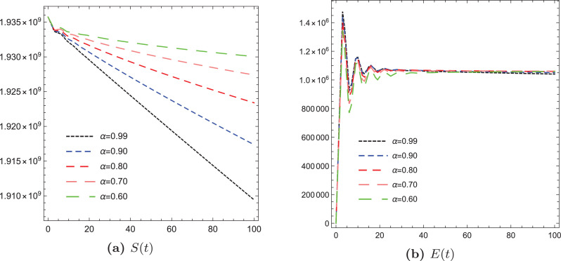
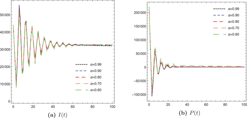
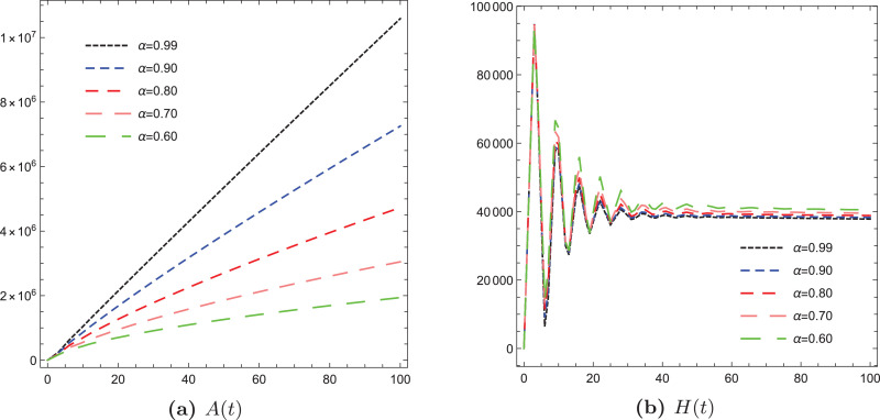
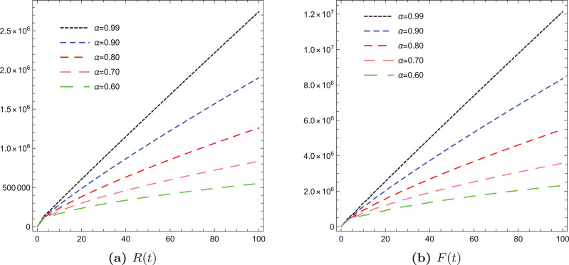
By simulating the above equations and as an illustration of the proposed numerical algorithm, we present some graphical illustrations for all variables of the new COVID-19 model in Fig. 5, Fig. 6, Fig. 7, Fig. 8 .

Fig. 5.

Illustrations of the variables S and E of the fractional COVID-19 model using different values of α.

Fig. 6.

Illustrations of the variables I and P of the fractional COVID-19 model using different values of α.

Fig. 7.

Illustrations of the variables A and H of the fractional COVID-19 model using different values of α.

Fig. 8.

Illustrations of the variables R and F of the fractional COVID-19 model using different values of α.

4. Conclusion

In the present paper, we presented a COVID-19 model with new fractional operator using ABFD. This mathematical and dynamical model is more suitable to describe the biological phenomena with memory than the integer order model. To test the behavior of all variables of the model, we simulated the resulting nonlinear fractional differential equations model by involving ABFD based on Daubechies framelet systems and obtained various graphical illustrations. It turns out that, increasing of the fractional value of the parameters resulting a decrease in the infection rates.

CRediT authorship contribution statement

Mutaz Mohammad: Conceptualization, Methodology, Visualization, Software, Investigation, Supervision, Validation, Writing - review & editing. Alexander Trounev: Software.

Declaration of Competing Interest

The authors declare that they have no known competing financial interests or personal relationships that could have appeared to influence the work reported in this paper.

References

- 1.Ghanbari B., Atangana A. A new application of fractional Atangana–Baleanu derivatives: designing ABC-fractional masks in image processing. Phys A. 2020;542:123516. [Google Scholar]
- 2.Atangana A., Bonyah E., Elsadany A. A fractional order optimal 4d chaotic financial model with Mittag-Leffler law. Chin J Phys. 2020;65:38–53. [Google Scholar]
- 3.Atangana A., Aguilar J., Kolade M., Hristov J. Fractional differential and integral operators with non-singular and non-local kernel with application to nonlinear dynamical systems. Chaos Solitons Fractals. 2020;132:109493. doi: 10.1016/j.chaos.2019.109493. [DOI] [Google Scholar]
- 4.Atangana A., Baleanu D. New fractional derivatives with nonlocal and non-singular kernel: theory and application to heat transfer model. Therm Sci. 2016;20:763–769. [Google Scholar]
- 5.Atangana A., Koca I. Chaos in a simple nonlinear system with atangana–Baleanu derivatives with fractional order. Chaos Solitons Fractals. 2016;89:447–454. [Google Scholar]
- 6.Atangana A. On the new fractional derivative and application to nonlinear Fisher’s reaction–diffusion equation. Appl Math Comput. 2016;273:948–956. [Google Scholar]
- 7.Atangana A., Aguilar J. Decolonisation of fractional calculus rules: breaking commutativity and associativity to capture more natural phenomena. Eur Phys J Plus. 2018;133:166. [Google Scholar]
- 8.Atangana A. Modelling the spread of COVID-19 with new fractal-fractional operators: can the lockdown save mankind before vaccination? Chaos Solitons Fractals. 2020;136(July):109860. doi: 10.1016/j.chaos.2020.109860. [DOI] [PMC free article] [PubMed] [Google Scholar]
- 9.Khan MA, Atangana A. Modeling the dynamics of novel coronavirus (2019-nCoV) with fractional derivative. 2020. In press.
- 10.Subashini R., Ravichandran C., Jothimani K., Baskonus H.M. Existence results of Hilfer integro-differential equations with fractional order. Discrete Contin Dyn Syst S. 2020;13(3):911–933. [Google Scholar]
- 11.Ndaïrou F., Area I., Nieto J., Torres D. Mathematical modeling of COVID-19, 205, transmission dynamics with a case study of Wuhan. Chaos Solitons Fractals. 2020:206. doi: 10.1016/j.chaos.2020.109846. [DOI] [PMC free article] [PubMed] [Google Scholar]
- 12.Mohammad M., Lin E.B. Gibbs phenomenon in tight framelet expansions. Commun Nonlinear Sci Numer Simul. 2018;55:84–92. [Google Scholar]
- 13.Mohammad M., Lin E.B. Contemporary mathematics. Vol. 706. AMS; 2018. Gibbs effects using daubechies and coiflet tight framelet systems; pp. 271–282. [Google Scholar]
- 14.Mohammad M. Special B-spline tight framelet and it’s applications. J Adv Math Comput Sci. 2018;29:1–18. [Google Scholar]
- 15.Mohammad M. On the Gibbs effect based on the quasi-affine dual tight framelets system generated using the mixed oblique extension principle. Mathematics. 2019;7(10):952. doi: 10.3390/math7100952. [DOI] [Google Scholar]
- 16.Mohammad M., Howari F., Acbas G., Nazzal Y., Al Aydaroos F. Wavelets based simulation and visualization approach for unmixing of hyperspectral data. Int J Earth Environ Sci. 2018;3 doi: 10.15344/2456-351X/2018/152. Article ID 3:IJEES-152, 8 pages. [DOI] [Google Scholar]
- 17.Mohammad M. Biorthogonal-wavelet-based method for numerical solution of Volterra integral equations M Mohammad. Entropy. 2019;21:1098. [Google Scholar]
- 18.Mohammad M. A numerical solution of Fredholm integral equations of the second kind based on tight framelets generated by the oblique extension principle. Symmetry. 2019;11:854. [Google Scholar]
- 19.Mohammad M., Cattani C. A collocation method via the quasi-affine biorthogonal systems for solving weakly singular type of volterra-fredholm integral equations. Alex Eng J. 2020 https://www.sciencedirect.com/science/article/pii/S1110016820300478. In press. [Google Scholar]
- 20.Mohammad M. Bi-orthogonal wavelets for investigating Gibbs effects via oblique extension principle. J Phys. 2020;1489 [Google Scholar]
- 21.Mohammad M., Cattani C.. Applications of bi-framelet systems for solving fractional order differential equations. 2020 Fractals. 10.1142/S0218348X20400514. [DOI]
- 22.Mohammad M. Bi-orthogonal wavelets for investigating Gibbs effects via oblique extension principle. J Phys. 2020;1489 [Google Scholar]
- 23.Mohammad M., Trounev A., Cattani C. The dynamics of COVID-19 in the UAE based on fractional derivative modeling using Riesz wavelets simulation, 05 June. 2020. PREPRINT (Version 1). 10.21203/rs.3.rs-33366/v1+. [DOI] [PMC free article] [PubMed]
- 24.Ravichandran C., Jothimani K., Baskonus H.M., Valliammal N. New results on nondensely characterized integro-differential equations with fractional order. Eur Phys J Plus. 2018;133(109):1–10. [Google Scholar]
- 25.Dokuyucu M.A., Celik E., Bulut H., Baskonus H.M. Cancer treatment model with the Caputo-Fabrizio fractional derivative. Eur Phys J Plus. 2018;133(92):1–7. [Google Scholar]
- 26.Yavuz M., Ozdemir N., Baskonus H.M. Solutions of partial differential equations using the fractional operator involving Mittag-Leffler kernel. Eur Phys J Plus. 2018;133(215):1–12. [Google Scholar]
- 27.Bulut H., Kumar D., Singh J., Swroop R., Baskonus H.M. Analytic study for a fractional model of HIV infection of CD4+TCD4+T lymphocyte cells. Math Nat Sci. 2018;2(1):33–43. [Google Scholar]
- 28.Mohammad Mutaz. An efficient method based on framelets for solving fractional volterra integral equations. Entropy. 2020;22(8):1–14. doi: 10.3390/e22080824. [DOI] [PMC free article] [PubMed] [Google Scholar]
- 29.Han B. Applied and numerical harmonic analysis. Birkhauser/Springer; Cham: 2017. Framelets and wavelets: algorithms, analysis, and applications. [Google Scholar]
- 30.Toufik M., Atangana A. New numerical approximation of fractional derivative with non-local and non-singular kernel: application to chaotic models. Eur Phys J Plus. 2017;132(10):444. [Google Scholar]