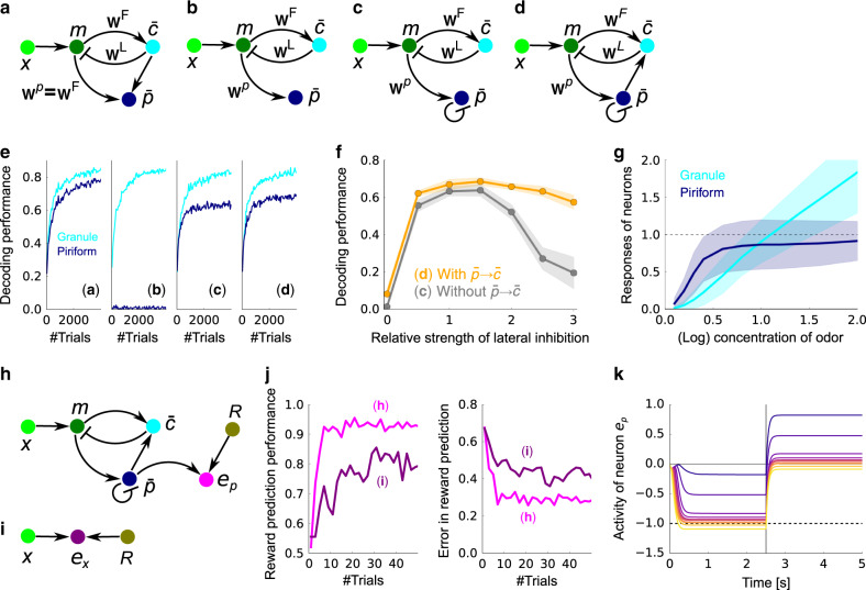
Fig. 7. Learning a concentration invariant representation and an odor-reward association.

a–d A set of increasingly realistic decoding models. a The decoding model associated with our variational Bayesian inference algorithm. Note that the weights need to be copied from w^F to w^p, something that is not biologically plausible. b Similar circuit, but with the mapping from m to $\overline{p}$ learned via a local rule. c Same as b, but with lateral inhibition. d Same as c, but with feedback to the granule cells. e Learning performance for the models in a–d when decoding from granule cells (cyan) or piriform cortex (dark blue; see subsection “Odor estimation performance” in the “Methods” section). f Comparison of performance for model c (gray) and d (orange). Mean and standard deviation over 10 simulations are plotted. g Mean and standard deviation of responses of the granule cells, $\overline{c}$, and the piriform neurons, $\overline{p}$, for their selective odors presented at various concentrations. The responses were measured by presenting each odor in isolation with different concentration, and then averaging over populations. h Schematic of the reward prediction circuit utilizing concentration-invariant representation in the piriform cells, $\overline{p}$. i Direct reward prediction from neural activity at glomeruli. j Performance of odor–reward association measured by the classification performance (left) and the mean-squared error between the predicted reward and the actual reward (right) for the models in panels h (magenta) and i (purple). Lines are mean over 100 simulations. k The mean response of neuron e_p given an odor associated with the reward. The vertical line at τ = 2.5 s represents the reward presentation, and the dotted horizontal line is the sign-flipped reward value (−R). Different colors represents the different concentrations of the presented odor, from purple (c ≈ 0.1) to yellow (c ≈ 2.0). In all panels, M = 50 odors, N = 200 glomeruli, and three odors were presented on average, except for the go/no go task where one of two selected odors was presented randomly.