Figure 1.

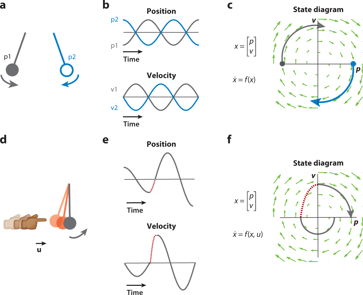
Example dynamics and population state of a frictionless pendulum. (a–c) A pendulum is a 2D dynamical system that has a simple relationship between the changes of the state of the pendulum (1D position and 1D velocity) and its current state. (a) Two example initial conditions are shown, p1 (gray; position is maximally negative and velocity is zero) and p2 (blue; position is maximally positive and velocity is zero). (b) As the pendulum moves through time, its state vector (position, top; velocity, bottom) is updated. (c) These trajectories can also be visualized by plotting one state variable against the other (position against velocity), beginning at the initial condition (circles) and moving along the flow field (green arrows), yielding the state space plot. The flow field shows the dynamical evolution of the pendulum for any set of initial conditions. (d–f) A pendulum with input perturbations. (d) One may perturb the pendulum during its motion, for example, by bumping it with a finger (brief period of the bumps appears in red). (e,f) This leads to a change in the pendulum state through time (red dashed lines) such that both the time series (e) and the state space trajectories (f) no longer follow the autonomous dynamics (as shown in panel e) while the input is active. After the perturbation is finished, the pendulum returns to its autonomous dynamics again (gray lines after red dashed lines). Figure adapted with permission from Pandarinath et al. (2018b).