
Figure 1. Mapping 3D genome with eHi-C.
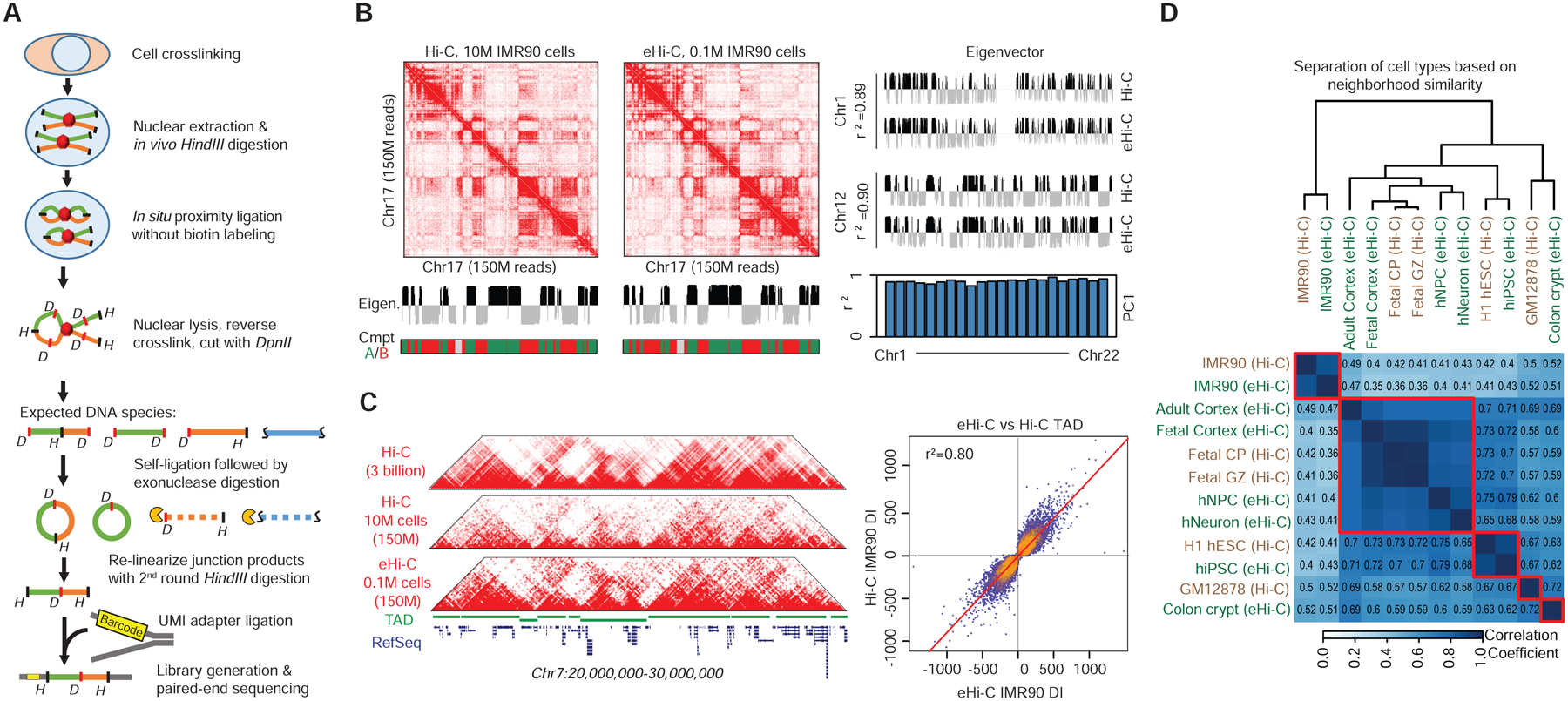
A, The scheme of eHi-C. B, Heatmaps show the contact matrices (Chr17) from Hi-C and eHi-C at 250kb resolution. The eigenvectors from Hi-C and eHi-C were very similar, leading to the same compartment A/B assignment. The comparison of eigenvectors between Hi-C and eHi-C in two other chromosomes are shown in the right panel. Histogram listed the r2 values of all chromosomes when comparing eigenvectors between eHi-C and Hi-C data. C, Heatmaps of contact matrices from Hi-C and eHi-C at 40kb resolution. The top track is drawn using a published IMR90 Hi-C dataset with ~3 billion reads. A track of TAD structures is plotted in green. On the right is a scatter plot comparing the directionality indexes (DI). The +/− sign of DI is used to determine TAD boundary. Very few bins change their signs of DI, indicating consistent TAD boundaries between Hi-C and eHi-C. D. Heatmap showing the similarity between 5 Hi-C and 7 eHi-C datasets (including a low-depth IMR90 eHi-C dataset) at compartment level. The correlation coefficient is computed by comparing the correlation matrices from different samples.