Figure 3. Microtubule growth rates as a function of microtubule plus-end density.

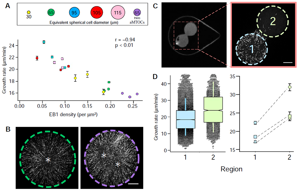
(A) Microtubule growth rates displayed as a function of EB1 comet density (see also Figure S2F). Error bars equal two SEMs. Pearson’s correlation coefficient (r) is indicated at the top of the graph and is significant if p < 0.01. (B) The effect of an additional aMTOC, with representative images showing EB1 signal from captured time-lapse series (see also Video S4). The left micro-enclosure (green dashed line) has one aMTOC, whereas the right micro-enclosure (purple dashed line) has two. Quantified microtubule growth rates are displayed in the graph in (A). Asterisks denote the relative positions of the aMTOCs (scale bar = 15 μm). (C) Hourglass-shaped micro-enclosure. The area indicated in the left panel is shown at higher magnification in the right panel and includes the two lobes of the hourglass enclosure (region 1 in light blue and region 2 in light green; scale bar = 15 μm). The left and right images were acquired from two different hourglass-shaped micro-enclosures. (D) Microtubule growth rates from the two regions of the hourglass micro-enclosures. The left graph displays grouped microtubule growth rates from the two regions of the micro-enclosure as box plots featuring a Tukey-style interquartile range (IQR), with whiskers indicating one SD of the median. Notches approximate the 95% confidence interval of the median for three different micro-enclosures. The right graph shows paired microtubule growth rates from the two regions of the hourglass micro-enclosure for three different enclosures. Error bars equal two SEMs. See also Figure S1.