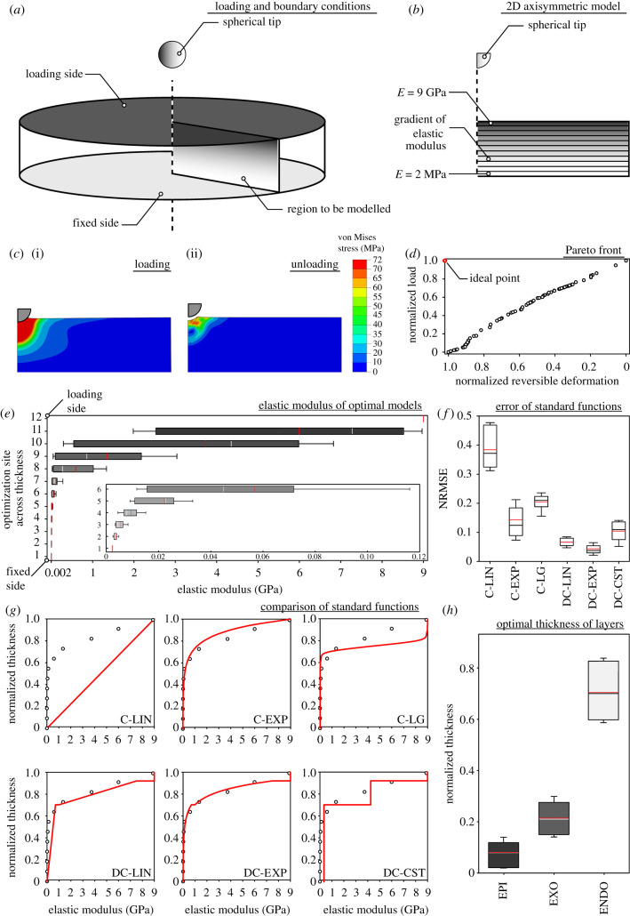
Figure 1.

Numerical simulation and optimization analysis. (a,b) Schematic diagram of the geometric model and indentation simulation. The geometric model (a) was reduced to an axisymmetric 2D model (b), which was fixed at the innermost layer and subjected to indentation with a spherical tip at the outermost surface. (c) Deformation and stress distribution in a representative model after loading (i) and after unloading (ii). (d) Distribution of optimal solutions along the Pareto front. (e) Distribution of the elastic modulus at 12 sites across the thickness of optimal models. The inset shows the enlarged view of the data for Sites 1–6. (f) NRMSE of six standard functions used to predict the optimal elastic modulus gradients. C-LIN, ‘continuous linear’ function; C-EXP, ‘continuous exponential’ function; C-LG, ‘continuous logistic’ function; DC-LIN, ‘discontinuous linear’ function; DC-EXP, ‘discontinuous exponential’ function; DC-CST, ‘discontinuous constant’ function. (g) Comparison between the mean optimal elastic modulus gradient (red line within the box in e) and six standard functions across the thickness of the geometric model. (h) Relative thickness of epi-, exo- and endocuticle in optimal models. EPI, epicuticle; ENDO, endocuticle; EXO, exocuticle. In all bar plots, the borders of the boxes indicate the 25th and 75th percentiles, a solid line (black/white) within them marks the median, a red line within them shows the mean and the whiskers (error bars) define the 10th and 90th percentiles.