Abstract
Ultrasonography is widely used in the clinical diagnosis of thyroid nodules. Ultrasound images of thyroid nodules have different appearances, interior features, and blurred borders that are difficult for a physician to diagnose into malignant or benign types merely through visual recognition. The development of artificial intelligence, especially deep learning, has led to great advances in the field of medical image diagnosis. However, there are some challenges to achieve precision and efficiency in the recognition of thyroid nodules. In this work, we propose a deep learning architecture, you only look once v3 dense multireceptive fields convolutional neural network (YOLOv3-DMRF), based on YOLOv3. It comprises a DMRF-CNN and multiscale detection layers. In DMRF-CNN, we integrate dilated convolution with different dilation rates to continue passing the edge and the texture features to deeper layers. Two different scale detection layers are deployed to recognize the different sizes of the thyroid nodules. We used two datasets to train and evaluate the YOLOv3-DMRF during the experiments. One dataset includes 699 original ultrasound images of thyroid nodules collected from a local health physical center. We obtained 10,485 images after data augmentation. Another dataset is an open-access dataset that includes ultrasound images of 111 malignant and 41 benign thyroid nodules. Average precision (AP) and mean average precision (mAP) are used as the metrics for quantitative and qualitative evaluations. We compared the proposed YOLOv3-DMRF with some state-of-the-art deep learning networks. The experimental results show that YOLOv3-DMRF outperforms others on mAP and detection time on both the datasets. Specifically, the values of mAP and detection time were 90.05 and 95.23% and 3.7 and 2.2 s, respectively, on the two test datasets. Experimental results demonstrate that the proposed YOLOv3-DMRF is efficient for detection and recognition of thyroid nodules for ultrasound images.
1. Introduction
With its ever-increasing incidence, the thyroid nodule is one of the most common nodular tumors in the adult population [1, 2]. The timely diagnosis of thyroid nodules is extremely essential. Ultrasonography is the primary and preferred screening method for the clinical diagnosis of thyroid nodules. The diagnosis comprises a fine needle aspiration biopsy (FNAB) and a follow-up treatment [3]. Clinically, doctors typically diagnose thyroid nodules by experience. However, this method could result in an ambiguous diagnosis [4], thereby causing excessive treatments such as unnecessary biopsy and surgery. With an increase in the number of patients, the radiologists are subjected to increased workloads. This may cause reduced average diagnostic time on each case, thereby leading to an increased incidence of misdiagnosis [5]. It is critical to accurately detect and recognize thyroid nodules as benign or malignant.
Traditionally, thyroid nodules have been mainly diagnosed visually, through human observation. However, it is difficult to accurately judge complicated thyroid nodules in ultrasound images through this method. Good old-fashioned artificial intelligence (GOFAI) and handcrafted features method [6] were developed to address the aforementioned problem. However, the two main drawbacks of GOFAI and the handcrafted features method are their high time complexity and unsatisfactory universality. The development of artificial intelligence, especially deep learning, has brought excellent advances in the field of medical image diagnosis. However, there are some challenges to achieve precision and efficiency in the recognition of thyroid nodules.
We propose a deep learning architecture, you only look once v3 dense multireceptive fields convolutional neural network (YOLOv3-DMRF), based on YOLOv3. It comprises a dense multireceptive fields convolutional neural network (DMRF-CNN) and multiscale detection layers. In DMRF-CNN, we integrate dilated convolution with different dilation rates to continue passing the edge and the texture features to deeper layers. Two different scale detection layers are deployed to recognize the different sizes of the thyroid nodules.
Figure 1 illustrates the frame diagram for the recognition of thyroid nodules. We use the ultrasound images of thyroid nodules as our dataset in the first stage. Subsequently, we process the original data through several operations that include the removal of artificial marks, image inpainting, and data augmentation. Lastly, the architecture YOLOv3-DMRF is presented to complete the detection and recognition.
Figure 1.

Frame diagram for recognition of thyroid nodules.
2. Related Work
In this section, we discuss some related works that focus on ultrasound images of thyroid nodules. They mainly comprise three stages: GOFAI, handcrafted features method [6], and deep learning method.
Initially, medical image analysis was performed with GOFAI or an expert system, which was similar to a rule-based image processing system. This method analyzed medical images by using low-level pixel processing and mathematical modeling method to solve tasks. Low-level pixel processing mainly included the following filters: edge detector, region growing, and line detector [7, 8]. Mathematical modeling mainly included fitting lines, circles, and ellipses [9]. However, the GOFAI approach was often brittle, and it required massive manual intervention.
Furthermore, several researchers used the handcrafted features method. For example, Toki and Tanaka [10] used the scale-invariant feature transform (SIFT) [11] to extract features in images to identify prostate cancer, whereas Niwas et al. [12] used the least squares support vector machine (LS-SVM) to diagnose breast cancer based on the texture characteristics of biopsy data. Furthermore, Basavanhally et al. [13] proposed a new multiview classifier on different sizes to identify the essential features of an image. These methods are based on the handcrafted features of pathological images of breast cancer. Nevertheless, the high variability of ultrasound images of thyroid nodules is a challenge in recognizing the benign or malignant types of the nodules. Moreover, in the case of changes in the characteristics such as distortion, clipping, lighting, and damage, the performances of these algorithms would worsen. Therefore, the universality on these previous methods is not stable.
Regarding the deep learning methods, the convolutional neural network (CNN) [14] was applied in image analysis, e.g., LeNet [15], AlexNet [16], visual geometry group network (VGGNet) [17], GoogLeNet [18], and residual network (ResNet) [19]. The CNN architecture can automatically extract the multilevel features. However, CNN for image classification progressively reduces resolution, which may further reduce the detailed spatial information. Dilated filters were developed in the à trous algorithm for efficient wavelet decomposition in [20], and they have been used in image pixel prediction to facilitate efficient computation [21, 22]. Comparison of the traditional convolutional kernel with the dilated convolution kernel of the same size shows that the latter requires a lesser number of network parameters, and it expands the receptive fields of the kernels to a greater degree to obtain almost the same information. Models based on dilated convolution have been actively explored for semantic segmentation of medical images. For example, Moeskops et al. [23] used dilated convolutions to segment images of brain MRI. The results showed improved segmentation performance while using the dilated convolutions procedure for segmentation of two different sets of images. Additionally, CNN has shown rapid development in image recognition, e.g., region-based CNN (R-CNN) [24], single shot detector (SSD) [25], Fast-RCNN [26], and Faster-RCNN [27]. However, these methods have high detection and recognition times. YOLO [28–30] is one of the state-of-the-art object detection systems designed by Joseph Redmon and Ali Farhadi. Compared to other object detection systems, the most outstanding feature of YOLO is high efficiency. YOLOv3, which is the third version, shows improved accuracy in addition to high efficiency. Therefore, YOLOv3 is used in our experiments.
Furthermore, some deep learning methods have been used in ultrasound images of thyroid nodules. For example, Chi et al. [31] used the fine-tuned GoogLeNet model to achieve good results on the open-access thyroid ultrasound image database [32]. Chi's method detected the location of thyroid nodules by manually gauging the position of the nodule, but failed to do so automatically. Li et al. [33] and Wang et al. [34] proposed an improved Fast R-CNN model for the detection of papillary thyroid carcinoma. Song et al. [35] proposed a multitask cascade CNN model by using SSD framework and a spatial pyramid network to detect thyroid nodules coarsely and finely, respectively. The aforementioned deep learning model can recognize thyroid nodules with a guaranteed satisfactory performance. However, the problems of complex network architectures with several parameters and large detection time cost must be solved urgently.
To address these problems, we present a deep learning architecture, YOLOv3-DMRF, based on YOLOv3, to detect and recognize thyroid nodules automatically and efficiently.
3. Data Preprocessing
3.1. Removal of Artificial Marks and Image Inpainting
Pathologists mark the outline of thyroid nodules during clinical diagnosis. This becomes a double-edged sword for the following reason. Although we can obtain the position and the size of nodules easily, additional noise is introduced during detection and recognition. Moreover, as shown in Figure 2, artificial marks merge into background pixels.
Figure 2.
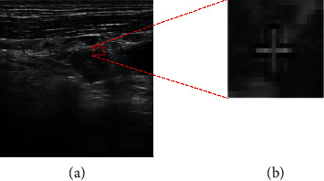
Ultrasound images of thyroid nodules with unclear artificial marks: (a) original image of having unclear artificial marks; (b) artificial marks are mixed with background pixels.
It is necessary to remove artificial marks in the preprocessing stage on the dataset. Based on numerous experiments, we use the Laplacian convolution [36] and the fast marching method (FMM) algorithm [37] to locate the positions of the artificial marks and remove them. Figure 3 illustrates the pipeline diagram of the processing. Firstly, the region of interest (ROI) of the ultrasound image is obtained. Subsequently, we use the Laplacian operator to find the locations of the artificial marks in the image. Next, we convert the input image into a binary one by using a reasonable threshold to obtain the artificial marks. Furthermore, we find the position of the marks in the original image based on the binary image and remove the marks. Finally, we perform the ultrasound image inpainting by using the INPAINT_TELEA algorithm of OpenCV [38].
Figure 3.

Ultrasonic image removal method and output.
3.2. Image Augmentation
To avoid overfitting, we use certain augmentation methods such as color jitter, change saturation, exposure, and hue to produce ultrasonic images as a supplement. It should be noted that we abandon the random transformation of angles because the aspect rate of thyroid nodules affects the discrimination between benign and malignant. In the experiments, we set jitter to 0.3, which represents that the ultrasonic images are randomly cropped and flipped using rates from 0 to 0.3. Meanwhile, we set both saturation and exposure to 1.5. The hue is 0.1, which represents the random generation of pictures in the range of −0.1 ∼ 0.1 hues.
4. YOLOv3-DMRF Model
In this work, we propose a deep learning architecture, YOLOv3-DMRF, for detection and recognition of thyroid nodules, as shown in Figure 4. It can be used in auxiliary diagnoses. Its depth is 81, and H and W denote the height and width of the feature maps, respectively. s (s = 1, 2, ..., 32) denotes the down-sampling rate the for the input images (416 × 416). Different colors represent feature maps with different operations. α denotes the dilation rate.
Figure 4.
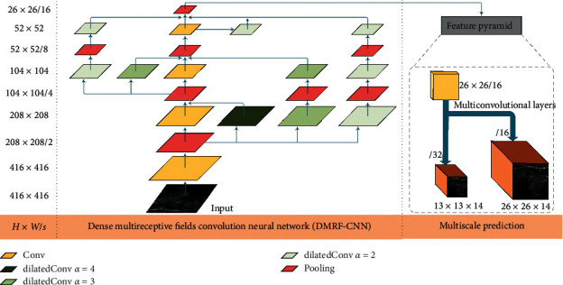
YOLOv3-DMRF architecture for thyroid nodules recognition.
4.1. IoU for Anchor Boxes
Object detection must choose anchor boxes in the training stage. In this work, we use the K-means algorithm to obtain original anchor boxes based on the training datasets that are derived from the original thyroid ultrasound images. Algorithm 1 outlines the procedure of the same. First, we randomly select K coordinates from the ground truth boxes set (gtbox) as the coordinates of the initial cluster centers: Ck, where k ∈ {1, 2, ..., K}. Furthermore, for the coordinates of the ground truth boxes, we calculate the distance to the K cluster centers and assign the coordinates to the set of the nearest center. This set is denoted as Csetk. Next, we calculate the mean of all the coordinates in cluster Csetk to update the coordinates of cluster center Ck. Finally, for the coordinates of all K cluster centers, we repeat the above steps until the coordinates of cluster center Ck do not change. The coordinates of the K cluster centers are the coordinates of the anchor boxes.
Algorithm 1.
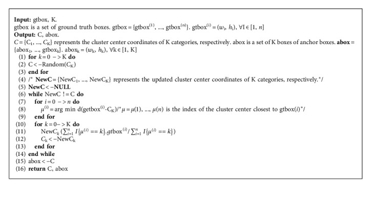
K-means get anchor box.
We use equation (1) to compute the distance between the K cluster centers for each of the other boxes:
| (1) |
Intersection over union (IoU) is a measure of the distance for two crossing objects, and it is defined as follows:
| (2) |
For each object bi, wi and hi are the width and the height, respectively. When the sizes of both the objects, b1 and b2, are equal, IoU reaches its maximum value of 1.
Additionally, to evaluate the effect of anchor box by the K-means algorithm, we calculate the average IoU (Avg IoU), which is defined as follows:
| (3) |
We set the number of clusters (K) to 4 after performing experiments, as shown in Table 1. We performed four sets of experiments, wherein the number of cluster centers (K) was set to 4, 6, 8, and 10. We found that K is proportional to Avg IoU. Moreover, it is well known that K is proportional to the detection time. Furthermore, we tested the Avg IoU (without the K-means algorithm) with the coordinates of the six cluster centers set by human experience. We found that the Avg IoU was 63.2%. Therefore, to improve the efficiency of the model, we chose K to be 4.
Table 1.
Avg IoU for K-means.
| K | 4 | 6 | 8 | 10 |
|---|---|---|---|---|
| Avg IoU (%) | 67.82 | 71.02 | 74.69 | 76.93 |
5. DMRF-CNN
Clinically, the edge and the texture features of thyroid nodules are the critical features for recognition of the benign or malignant type of the nodules. To extract the edge and the texture features, we present DMRF-CNN that uses dilated convolution [39] and cross-layer connections. The details of DMRF-CNN are provided in Figure 5. The label, d-x-conv-y, indicates dilated convolution, where x is the dilation rate and y denotes the convolution layer. Conv represents a traditional convolution. Cx represents the name of a connection. Different colors represent the feature maps with different operations.
Figure 5.
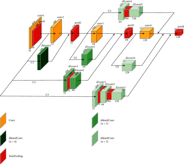
Structure and detailed parameters of DMRF-CNN.
We combine the traditional convolution (dilation rate of 1) with dilated convolution in DMRF-CNN. Dilated convolution can enlarge the receptive fields with various dilation rates. Different dilation rates correspond to different convolution kernel sizes. We use the batch normalization and the leaky rectified linear unit (Leaky ReLU) layers after the dilated convolution layer to avoid gradient disappearance. We term the aforementioned dilated operation as the dilatedConv block. In the experiments in this study, we used three dilation rates: 4, 3, and 2, as shown in Figure 6. Furthermore, we use high dilation rate in the shallow layers and low in deep layers. The value of the parameter of the Leaky ReLU is 0.1.
Figure 6.

Different kernel sizes corresponding to different dilation rates (here, the 3 × 3 convolution kernel size is considered as an example): (a) the dilation rate is 1(conventional convolution kernel); (b) the dilation rate is 2; (c) the dilation rate is 3; (d) the dilation rate is 4.
In this work, dense connections are deployed to improve the information transmission between different layers. We use the add operation that adds feature maps to connect two feature maps. For example, the maps: d4conv1 and conv2 are connected by an add operation. We perform max pooling down-sampling to ensure that the feature maps have the same size before the add operation. The dimensions of the feature map after pool4 are 26 × 26 × 128.
5.1. Detection and Recognition
Based on the feature maps encoded by the DMRF-CNN, we achieve the detection and classification of thyroid nodules. In this work, two scales are considered to recognize the nodules of different sizes. For each scale, we set two bounding boxes. A tuple comprising four items, i.e., (x, y, w, and h) is used to present a bounding box. Here, x and y denote the relative coordinates of the center of the bounding box. Furthermore, wand h denote the width and height of the box, respectively. We use confidence to evaluate the accuracy of detection, which is computed by as
| (4) |
IoU(T, P) denotes the IoU of the ground truth and the prediction bounding box. Each thyroid nodule original image is divided into different scale grid cells. In this study, we obtain two scales division: by 13 × 13 and 26 × 26. Two anchor boxes are set for each scale. For each grid cell, we predict two bounding boxes. ∂ has two values: 1 and 0. If the center points of the ground truths are in the current grid cell, ∂ = 1; otherwise, ∂ = 0.
In this work, we use a tensor comprising x, y, w, h, confidence, and the classification probability for each bounding box, as shown in Figure 7. For each scale recognition, we form a 1 × 1 × 14 evaluation. Here, C1 and C2 denote the prediction probability for the benign and malignant states, respectively. Based on the prediction bounding boxes, we use the nonmaximum suppression (NMS) algorithm [40] to ensure that one thyroid nodule has only one bounding box.
Figure 7.
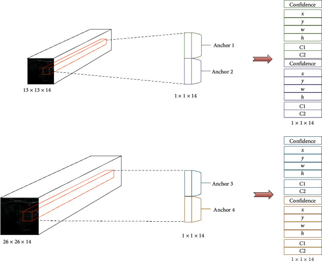
Channel design of detection layers.
The loss function of YOLOv3-DMRF has three parts: classification loss, localization loss, and confidence loss, which are shown by equation (5). In equation (5), s2 denotes the number of divided grid cells with B bounding boxes for each grid cell. μweight and μnoboj denote the contribution rate. μweight can increase the difference in the localization loss, whereas μnoboj can decrease the loss from the confidence predictions for the bounding boxes that do not contain thyroid nodules. In the experiment, we set μweight = 5 and μnoboj = 0.5. Conf denotes the confidence, as shown in equation (4). Furthermore, p(c) refers to the classification prediction. τiobj is 1 if object appears in the ith grid cell; otherwise, the result is 0. The value of τijobjis 1 if the jth bounding box predictor is in ith grid cell; otherwise, 0:
| (5) |
6. Results and Discussion
6.1. Experimental Setup
6.1.1. Datasets and Evaluation Metrics
The dataset used in this study was obtained from 240 patients with 699 ultrasound images of thyroid nodules, which were followed by FNAB. They were collected from the physical health center of a local 3A hospital. These ultrasound images belong to 34 males and 177 females. In our dataset, each image contains at least one thyroid nodule. There are 360 benign and 486 malignant nodules. A total of 10,485 images were obtained through data augmentation. Details of the training and test datasets are provided in Table 2.
Table 2.
Details of training and test datasets.
| Training dataset | Test dataset | Total | |
|---|---|---|---|
| Original datasets | 490 | 209 | 699 |
| Augmented datasets | 10276 | 209 | 10485 |
In the experiment, we used the metrics: average precision (AP) and mean average precision (mAP) to evaluate the detection and recognition of thyroid nodules. In addition, we use f1 score, recall, accuracy, and precision to evaluate the classification performance of thyroid nodules. They are calculated as follows:
| (6) |
| (7) |
where N represents the total number of images in the test sets, P(n) is the value of precision, and ∆r(n) denotes the recall value. The metric, mAP, represents the average of multiple categories of APs, and M is the number of classifications:
| (8) |
| (9) |
| (10) |
| (11) |
where TP, TN, FP, and FN represent true positives (TP), true negatives (TN), false positives (FP), and true negatives (FN), respectively.
6.1.2. Parameter Setup
The experiments in this study are based on the improved YOLOv3 object detection framework. We used a random gradient descent (SGD) for 60 K iteration training with an initial learning rate of 0.01 and a batch size of 16 images. At the iterations of 40 K and 50 K, the learning rate is reduced by 10 times. To demonstrate the efficiency of YOLOv3-DMRF, we compared it with some state-of-the-art networks based on YOLOv3 such as YOLOv3-tiny, YOLOv3-spp, YOLOv3-320, YOLOv3-416, and YOLOv3-608 on our and an open-access dataset. YOLOv3-spp denotes spatial pyramid pooling (SPP) based on YOLOv3. YOLOv3-320, YOLOv3-416, and YOLOv3-608 represent the different input shapes for DarkNet based on YOLOv3. Furthermore, we also compared the effects of different layer connections and different dilation rates on the precision of the framework. Moreover, we compared the feature maps of different dilation rates to obtain the results of different dilation rates. And we compared the proposed DMRF-CNN with some state-of-the-art CNN models to better demonstrate the performance on the same metrics.
6.2. Results and Analysis
6.2.1. Evaluation of Layer Connection and Different Dilation Rates
We compare different dilation rates, as shown in Table 3. In this experiment, we set each convolution as a dilated convolution, and the dilation rates are listed in Table 3. It is evident that, compared with traditional convolution, the mAP improves on using dilated convolution. The mAP shows the best value when the dilation rate is 2.
Table 3.
mAP of different dilation rates.
| Dilation rate | 1 | 2 | 3 | 4 |
|---|---|---|---|---|
| mAP (%) | 85.06 | 88.95 | 87.61 | 84.68 |
In this work, we evaluate the layer connection on the dilated convolution (dilation rate is 1) operations. Here, six different connections are used as shown in Table 4. The mean values of Cx are shown in Figure 5. As seen in Table 4, six group experiments are developed to evaluate the layer connection. The results show that the optimal mAP is achieved when all six connection methods are used.
Table 4.
mAP of different connections.
| Name | C1 | C2 | C3 | C4 | C5 | C6 | mAP (%) |
|---|---|---|---|---|---|---|---|
| I | 85.06 | ||||||
| II | ∗ | ∗ | ∗ | 85.37 | |||
| III | ∗ | ∗ | 84.72 | ||||
| IV | ∗ | ∗ | ∗ | ∗ | ∗ | 84.99 | |
| V | ∗ | ∗ | ∗ | ∗ | 85.01 | ||
| VI | ∗ | ∗ | ∗ | ∗ | ∗ | ∗ | 85.43 |
According to Table 4, experiment VI reaches the best performance. Thus, we combine this full layer connection with different dilation rates in follow-up experiments. Different dilation rates will correspond to different results on the layer connection. And the specific results are shown in Table 5. Specifically, the experiments I, II, and III only combine two different dilation rates, and the mAP increases by 2.89%, 1.53%, and 1.99%, respectively, compared to the 85.43% (Table 4, VI). These results revalidate that adding dilated convolution can increase the performance to some extent. In other experiments, we try to fuse dilation rates of no less than three various combinations. It is clear that VII fusion with the four different dilation ratios outperforms other fusions. We employ the structure of the VII model to construct the YOLOv3-DMRF framework.
Table 5.
mAP of fusion of different dilation rates.
| Name | Dilation rate = 1 | Dilation rate = 2 | Dilation rate = 3 | Dilation rate = 4 | MAP (%) |
|---|---|---|---|---|---|
| I | ∗ | ∗ | 88.32 | ||
| II | ∗ | ∗ | 86.96 | ||
| III | ∗ | ∗ | 87.42 | ||
| IV | ∗ | ∗ | ∗ | 88.54 | |
| V | ∗ | ∗ | ∗ | 87.91 | |
| VI | ∗ | ∗ | ∗ | 89.54 | |
| VII | ∗ | ∗ | ∗ | ∗ | 90.05 |
Figure 8 presents the comparisons between the traditional (dilation rate = 1) and the dilated convolutions (dilation rate = 4, 3, 2). It presents the feature maps generated by convolution kernels with different dilation rates. Here, conv2 is the traditional convolution, and d4conv1, d3conv1, and d2conv1 are the dilated convolutions for rates 4, 3, and 2, respectively. It is evident that the dilated convolutions outperform the traditional one on the extraction of texture and edge features.
Figure 8.
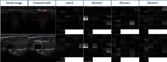
Comparisons between traditional and dilated convolutions.
6.2.2. Evaluation of DMRF-CNN on Our Dataset
To better validate the feasibility of the designed DMRF-CNN architecture, we also retain some state-of-the-art networks on our thyroid dataset. For the dataset, we split it refer to above Table 2. Before training, we crop and resize the thyroid nodules of ultrasound images to the same size (240 ∗ 240). To quickly attain the convergence of every model, we utilize SGD as the optimizer and employ cross-entropy as the loss function. Table 6 describes specific comparisons between DMRF-CNN and these structures on four metrics the classification accuracy, f1 score, precision, and recall. DMRF-CNN achieves the best performance on all four metrics, especially for the recall (97.39%). For other models, we conclude that DarkNet shows stability and reaches the same level on these metrics. The precision on DarkNet is 88.39%, ranking second behind the DMRF-CNN. However, the densely connected convolutional networks (DenseNet) [41] obtain the disappointing results on all metrics except the precision, showing the fluctuation. Meanwhile, Figure 9 illustrates the corresponding ROC curves. Each color represents each network architecture. It is clear that our proposed method DMRF-CNN gets the best performance and the AUC is 95.3%. The AUC value of DarkNet is 0.853, which is only behind DMRF-CNN. This again demonstrates the stability of the DarkNet, even if it cannot keep up with the AUC of DMRF CNN. Similarly, the worst value is still DenseNet, and our method ranks 22.1 percentage points higher in the AUC than it.
Table 6.
The metrics of DMRF-CNN and some state-of-the-art networks.
Figure 9.
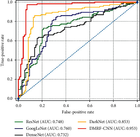
The ROC curve of DMRF-CNN and some state-of-the-art networks.
6.2.3. Evaluation of Different Models on Our Dataset
As shown in Table 7, we compare the mAP for YOLOv3-DMRF with that of the state-of-the-art-models based on YOLOv3. It is seen that YOLOv3-416 achieves mAP of 90.58% and the detection time is 9 s. This could be caused by the model depth of 106. The YOLOv3-DMRF model achieves mAP of 90.05%, and the detection time is very short, i.e., 3.7 s. As shown in Figure 10, the benign and malignant AP values of YOLOv3-320, YOLOv3-416, and YOLOv3-608 achieve AP values for benign and malignant types; however, the cost of detection time is very high than that of YOLOv3-DMRF. Compared to other models, the mAP of YOLOv3-DMRF does not differ much; however, its detection speed is three times greater.
Table 7.
mAP of different networks on our dataset.
| Model | Benign (AP) (%) | Malignant (AP) (%) | Detection time in all test images (s) | mAP on our dataset (%) |
|---|---|---|---|---|
| YOLOv3-tiny | 79.50 | 89.86 | 2 | 84.68 |
| YOLOv3-spp | 79.43 | 63.30 | 11.3 | 71.36 |
| YOLOv3-320 | 90.91 | 90.18 | 9.1 | 90.54 |
| YOLOv3-416 | 90.91 | 90.26 | 9.4 | 90.58 |
| YOLOv3-608 | 90.79 | 89.86 | 9.8 | 90.32 |
| YOLOv3-DMRF | 90.66 | 89.43 | 3.7 | 90.05 |
Figure 10.
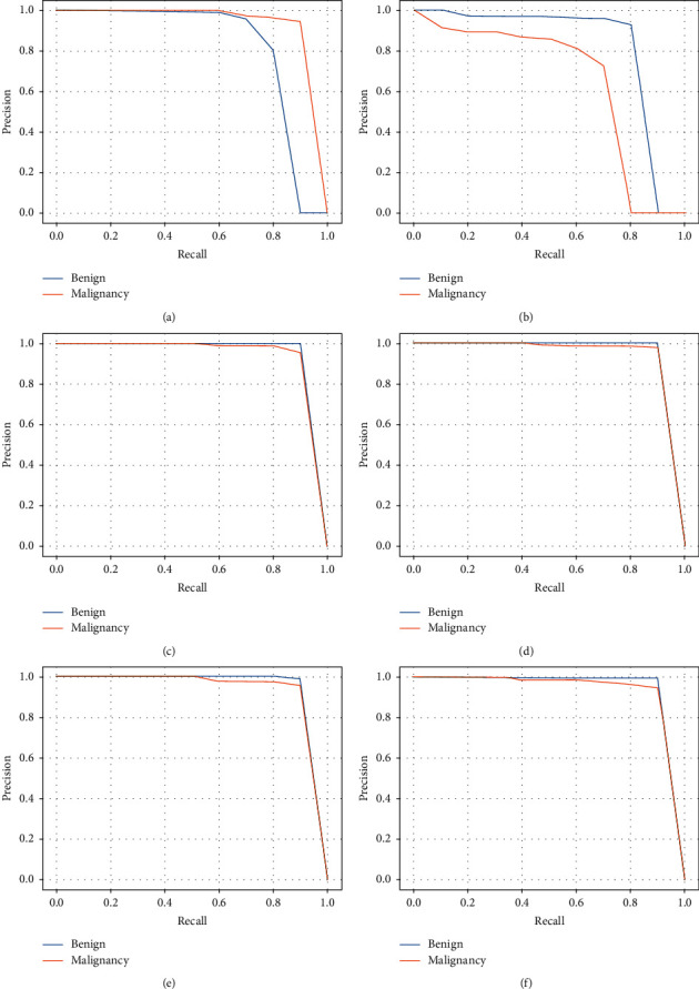
PR curve of different methods: (a) PR curve of YOLOv3-tiny; (b) PR curve of YOLOv3-spp; (c) PR curve of YOLOv3-320; (d) PR curve of YOLOv3-416; (e) PR curve of YOLOv3-608; (f) PR curve of YOLOv3-DMRF.
Furthermore, we compare the performance of YOLOv3-DMRF with other object detection algorithms, as shown in Table 8. Through this data analysis, we may draw the conclusion, our proposed method is not only higher in mAP than other object detection frameworks but also better in detection time. Our proposed method has the same AP between benign and malignant; thus, our model is far more stable than other object detection frameworks that owe high AP on malignant because the detection algorithms cannot detect small nodules that are usually diagnosed with benign nodules. In addition, inspired by the one-stage structure of SSD and YOLOv3-DMRF, their detection time outperforms the Fast R-CNN. In addition, we draw the PR curve of three methods in Figure 11. It is seen that our proposed methods outperform other methods in the AP number on different classes. The low diversity of YOLOv3-DMRF between the two categories cannot be ignored.
Table 8.
Evaluation of YOLOv3-DMRF and other object detection on our dataset.
Figure 11.
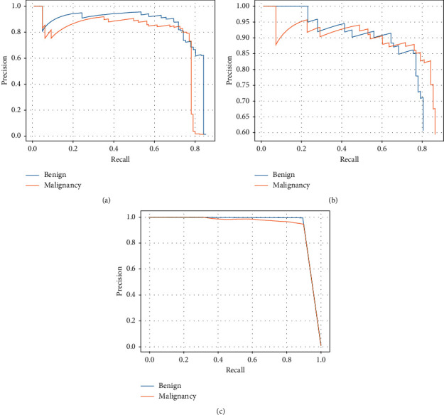
The PR curves of YOLOv3-DMRF and some object detection methods: (a) PR curve of Fast R-CNN; (b) PR curve of SSD; (c) PR curve of YOLOv3-DMRF.
6.2.4. Evaluation on Open-Access Datasets
In this work, we evaluate the universality of YOLOv3-DMRF on open datasets [32]. The open-access dataset includes 299 patients, of whom 270 are women and 29 are men. We treat the labels 4c and 5 in this open-access dataset as the malignant nodules while others as benign ones. We acquired 111 malignant and 41 benign thyroid nodules. As shown in Table 9, our network outperforms other state-of-the-art networks based on YOLOv3.
Table 9.
mAP of different networks for an open-access dataset.
| Model | Benign (AP) (%) | Malignant (AP) (%) | Detection time in all test images (s) | mAP (%) |
|---|---|---|---|---|
| YOLOv3-tiny | 72.73 | 80.72 | 0.9 | 76.72 |
| YOLOv3-spp | 49.59 | 57.88 | 9 | 53.73 |
| YOLOv3-320 | 72.73 | 89.87 | 4.5 | 81.3 |
| YOLOv3-416 | 72.73 | 98.04 | 4.9 | 85.38 |
| YOLOv3-608 | 79.97 | 89.83 | 8 | 84.85 |
| YOLOv3-DMRF | 92.68 | 97.59 | 2.2 | 95.23 |
Furthermore, we evaluate the mAP with different object detection methods on the open-access dataset. As shown in Table 10, we can see that the detection time and mAP of our methods outperform other methods. At the same time, the AP number of two classes is stable, and the AP number is 92.68% and 97.59%, respectively.
Table 10.
Evaluation of YOLOv3-DMRF and other object detection on open-access dataset.
6.2.5. Visualization
In this work, we present four images (two images from our dataset and two images from the open dataset) of thyroid nodules. The results of the recognition are shown in Figure 12. In the first and second columns are test images from our dataset, and we can see that the bounding box of Fast R-CNN method outperforms the SSD method, but the classification and detection time of SSD outperforms Fast R-CNN. The bounding box of the YOLOv3-DMRF method is not only close to the ground truth but also the classification outperforms Fast R-CNN and SSD methods. Especially, the accuracy of our method is 6.3 percentage points higher than Fast R-CNN for benign nodules because our proposed method used a multidetection layer. In the public dataset, we can see that the Fast R-CNN and SSD methods cannot detect the benign nodule, but YOLOv3-DMRF can detect this nodule and the accuracy of classification is 100 percent.
Figure 12.
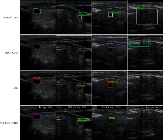
Detection using our method and other object detection methods. The first and second columns are test images form our dataset, and the last two columns are test images from open dataset.
7. Conclusions
In this paper, we proposed YOLOv3-DMRF, based on YOLOv3, to detect and recognize thyroid nodules efficiently. We presented DMRF-CNN to extract the edge and the texture features of thyroid nodules. Especially, we compared some state-of-the-art CNN models. The results showed that DMRF-CNN has a good stability, and the AUC number is 95.3% in our dataset. We used a multiscale detection layer to recognize different sizes of the nodules. The experimental results showed that YOLOv3-DMRF outperforms other models on performance and detection time, and mAP was 90.05% on our dataset. Moreover, we evaluated YOLOv3-DMRF on an open-access dataset, where it achieved good mAP and detection time. The mAP was 95.23%, and the detection time was 2.2 s, which are very good compared to other models. In future, we will continue to collect ultrasound images of thyroid nodules to improve the mAP of our method. Additionally, we plan to further classify the malignant nodules by using ultrasound images.
Acknowledgments
Firstly, the authors thank Cooperative Innovation Center of Internet Healthcare, Zhengzhou University (ih.ha.edu.cn), for providing the platform on cooperative innovation for medical and engineering. Secondly, the authors thank the Department of Health Management, Henan Provincial People's Hospital, for providing the original thyroid ultrasound images and medical knowledge for the detection and recognition of thyroid nodules. This work was supported by the Program of Scientific and Technological Research of Henan Province (grant number 192102310215), the Program of Key Science and Technological Research of Henan Province (grant number 18A520049), and the Program of Henan Medical Science and Technology Research Project (grant number 201702155).
Data Availability
The collected data used to support the findings of this study are restricted by the Department of Health Management, Henan Provincial People's Hospital in order to protect patient privacy. The collected data are available from Runzhi Li via rzli@ha.edu.cn for researchers who meet the criteria for access to confidential data. The open-access data used to support the findings of this study are included within the article.
Conflicts of Interest
The authors declare that there are no conflicts of interest.
Authors' Contributions
Jingzhe Ma and Shaobo Duan contributed equally to this work.
References
- 1.Jin H., Yan H., Tang H., Zheng M., Wu C., Liu J. Internal spreading of papillary thyroid carcinoma: a case report and systemic review. Case Reports in Endocrinology. 2018;2018:5. doi: 10.1155/2018/7618456.7618456 [DOI] [PMC free article] [PubMed] [Google Scholar]
- 2.Sanabria A., Kowalski L. P., Shah J. P., et al. Growing incidence of thyroid carcinoma in recent years: factors underlying overdiagnosis. Head & Neck. 2018;40(4):855–866. doi: 10.1002/hed.25029. [DOI] [PMC free article] [PubMed] [Google Scholar]
- 3.Ventura M., Melo M., Carrilho F. Selenium and thyroid disease: from pathophysiology to treatment. International Journal of Endocrinology. 2017;2017:9. doi: 10.1155/2017/1297658.1297658 [DOI] [PMC free article] [PubMed] [Google Scholar]
- 4.Liu Y., Su L., Xiao H. Review of factors related to the thyroid cancer epidemic. International Journal of Endocrinology. 2017;2017:9. doi: 10.1155/2017/5308635.5308635 [DOI] [PMC free article] [PubMed] [Google Scholar]
- 5.Park C. S., Kim S. H., Jung S. L., et al. Observer variability in the sonographic evaluation of thyroid nodules. Journal of Clinical Ultrasound. 2010;38(6):287–293. doi: 10.1002/jcu.20689. [DOI] [PubMed] [Google Scholar]
- 6.Litjens G., Kooi T., Bejnordi B. E., et al. A survey on deep learning in medical image analysis. Medical Image Analysis. 2017;42:60–88. doi: 10.1016/j.media.2017.07.005. [DOI] [PubMed] [Google Scholar]
- 7.Harris C. G., Stephens M. A combined corner and edge detector. Proceedings of the Alvey Vision Conference; September 1988; Manchester UK. Citeseer; pp. 10–5244. [Google Scholar]
- 8.Kulikowski J. J., King-Smith P. E. Spatial arrangement of line, edge and grating detectors revealed by subthreshold summation. Vision Research. 1973;13(8):1455–1478. doi: 10.1016/0042-6989(73)90006-0. [DOI] [PubMed] [Google Scholar]
- 9.Fitzgibbon A., Pilu M., Fisher R. B. Direct least square fitting of ellipses. IEEE Transactions on Pattern Analysis and Machine Intelligence. 1999;21(5):476–480. doi: 10.1109/34.765658. [DOI] [Google Scholar]
- 10.Toki Y., Tanaka T. Image feature extraction method with SIFT to diagnose prostate cancer. Proceedings of SICE Annual Conference (SICE); August 2012; Akita, Japan. IEEE; pp. 2185–2188. [Google Scholar]
- 11.Lowe D. G. Distinctive image features from scale-invariant keypoints. International Journal of Computer Vision. 2004;60(2):91–110. doi: 10.1023/b:visi.0000029664.99615.94. [DOI] [Google Scholar]
- 12.Niwas S. I., Palanisamy P., Zhang W., Isa N. A. M., Chibbar R. Log-gabor wavelets based breast carcinoma classification using least square support vector machine. Proceedings of the IEEE International Conference on Imaging Systems and Techniques; May 2011; Penang, Malaysia. IEEE; pp. 219–223. [Google Scholar]
- 13.Basavanhally A., Ganesan S., Feldman M., et al. Multi-field-of-view framework for distinguishing tumor grade in ER+ breast cancer from entire histopathology slides. IEEE Transactions on Biomedical Engineering. 2013;60(8):2089–2099. doi: 10.1109/tbme.2013.2245129. [DOI] [PMC free article] [PubMed] [Google Scholar]
- 14.Fukushima K. Neocognitron: a self-organizing neural network model for a mechanism of pattern recognition unaffected by shift in position. Biological Cybernetics. 1980;36(4):193–202. doi: 10.1007/bf00344251. [DOI] [PubMed] [Google Scholar]
- 15.LeCun Y., Bottou L., Bengio Y., Haffner P. Gradient-based learning applied to document recognition. Proceedings of the IEEE. 1998;86(11):2278–2324. doi: 10.1109/5.726791. [DOI] [Google Scholar]
- 16.Krizhevsky A., Sutskever I., Hinton G. E. Imagenet classification with deep convolutional neural networks. Proceedings of the Advances in Neural Information Processing Systems; December 2012; Lake Tahoe, NV, USA. NIPS; pp. 1097–1105. [Google Scholar]
- 17.Simonyan K., Zisserman A. Very deep convolutional networks for large-scale image recognition. 2014. http://arxiv.org/abs/1409.1556.
- 18.Szegedy C., Liu W., Jia Y., et al. Going deeper with convolutions. Proceedings of the IEEE Conference on Computer Vision and Pattern Recognition; October 2015; Boston, MA, USA. IEEE; pp. 1–9. [Google Scholar]
- 19.He K., Zhang X., Ren S., Sun J. Deep residual learning for image recognition. Proceedings of the IEEE Conference on Computer Vision and Pattern Recognition; December 2016; Las Vegas, NV, USA. IEEE; pp. 770–778. [Google Scholar]
- 20.Holschneider M., Kronland-Martinet R., Morlet J., Tchamitchian P. Wavelets. New York, NY, USA: Springer; 1990. A real-time algorithm for signal analysis with the help of the wavelet transform; pp. 286–297. [Google Scholar]
- 21.Giusti A., Cireşan D. C., Masci J., Gambardella L. M., Schmidhuber J. Fast image scanning with deep max-pooling convolutional neural networks. Proceedings of the IEEE International Conference on Image Processing; September 2013; Melbourne, Australia. IEEE; pp. 4034–4038. [Google Scholar]
- 22.Sermanet P., Eigen D., Zhang X., Mathieu M., Fergus R., LeCun Y. Overfeat: integrated recognition, localization and detection using convolutional networks. 2013. http://arxiv.org/abs/1312.6229.
- 23.Moeskops P., Veta M., Lafarge M. W., Eppenhof K. A., Pluim J. P. Deep Learning in Medical Image Analysis and Multimodal Learning for Clinical Decision Support. Newyork, NY, USA: Springer; 2017. Adversarial training and dilated convolutions for brain MRI segmentation; pp. 56–64. [Google Scholar]
- 24.Girshick R., Donahue J., Darrell T., Malik J. Rich feature hierarchies for accurate object detection and semantic segmentation. Proceedings of the IEEE Conference on Computer Vision and Pattern Recognition; June 2014; Columbus, OH, USA. IEEE; pp. 580–587. [Google Scholar]
- 25.Liu W., Anguelov D., Erhan D., et al. SSD: single shot multibox detector. Proceedings of the European Conference on Computer Vision; October 2016; Amsterdam, Netherlands. Springer; pp. 21–37. [Google Scholar]
- 26.Girshick R. Fast R-CNN. Proceedings of the IEEE International Conference on Computer Vision; December 2015; Santiago, Chile. IEEE; pp. 1440–1448. [Google Scholar]
- 27.Ren S., He K., Girshick R., Sun J., Faster R-CNN. Towards real-time object detection with region proposal networks. Advances in Neural Information Processing Systems. 2015:91–99. [Google Scholar]
- 28.Redmon J., Divvala S., Girshick R., Farhadi A. You only look once: unified, real-time object detection. Proceedings of the IEEE Conference on Computer Vision and Pattern Recognition; June 2016; Las Vegas, NV, USA. IEEE; pp. 779–788. [Google Scholar]
- 29.Redmon J., Farhadi A. YOLO9000: better, faster, stronger. Proceedings of the IEEE Conference on Computer Vision and Pattern Recognition; July 2017; Honolulu, HI, USA. IEEE; pp. 7263–7271. [Google Scholar]
- 30.Redmon J., Farhadi A. Yolov3: an incremental improvement. 2018. http://arxiv.org/abs/1804.02767.
- 31.Chi J., Walia E., Babyn P., Wang J., Groot G., Eramian M. Thyroid nodule classification in ultrasound images by fine-tuning deep convolutional neural network. Journal of Digital Imaging. 2017;30(4):477–486. doi: 10.1007/s10278-017-9997-y. [DOI] [PMC free article] [PubMed] [Google Scholar]
- 32.Pedraza L., Vargas C., Narváez F., Durán O., Muñoz E., Romero E. An open access thyroid ultrasound image database. Proceedings of the 10th International Symposium On Medical Information Processing And Analysis; October 2015; Cartagena de Indias, Columbia. International Society for Optics and Photonics; p. p. 92870W. [Google Scholar]
- 33.Li H., Weng J., Shi Y., et al. An improved deep learning approach for detection of thyroid papillary cancer in ultrasound images. Scientific Reports. 2018;8(1):p. 6600. doi: 10.1038/s41598-018-25005-7. [DOI] [PMC free article] [PubMed] [Google Scholar]
- 34.Wang Y., Ke W., Wan P. A method of ultrasonic image recognition for thyroid papillary carcinoma based on deep convolution neural network. NeuroQuantology. 2018;16(5) doi: 10.14704/nq.2018.16.5.1306. [DOI] [Google Scholar]
- 35.Song W., Li S., Liu J., et al. Multitask cascade convolution neural networks for automatic thyroid nodule detection and recognition. IEEE Journal of Biomedical and Health Informatics. 2018;23(3):1215–1224. doi: 10.1109/JBHI.2018.2852718. [DOI] [PubMed] [Google Scholar]
- 36.Narendra V., Hareesha K. Study and comparison of various image edge detection techniques used in quality inspection and evaluation of agricultural and food products by computer vision. International Journal of Agricultural & Biological Engineering. 2011;4(2):83–90. [Google Scholar]
- 37.Telea A. An image inpainting technique based on the fast marching method. Journal of Graphics Tools. 2004;9(1):23–34. doi: 10.1080/10867651.2004.10487596. [DOI] [Google Scholar]
- 38.Pulli K., Baksheev A., Kornyakov K., Eruhimov V. Real-time computer vision with openCV. Communications of the ACM. 2012;55(6):61–69. doi: 10.1145/2184319.2184337. [DOI] [Google Scholar]
- 39.Yu F., Koltun V. Multi-scale context aggregation by dilated convolutions. 2015. arXiv preprint arXiv:1511.07122.
- 40.Neubeck A., Van Gool L. Efficient non-maximum suppression. Proceedings of the 18th International Conference On Pattern Recognition (ICPR’06); August 2006; Hong Kong, China. IEEE; pp. 850–855. [Google Scholar]
- 41.Huang G. Densely connected convolutional networks. Proceedings of the IEEE Conference on Computer Vision and Pattern Recognition; December 2018; Las Vegas, NV, USA. IEEE; pp. 4700–4708. [Google Scholar]
Associated Data
This section collects any data citations, data availability statements, or supplementary materials included in this article.
Data Availability Statement
The collected data used to support the findings of this study are restricted by the Department of Health Management, Henan Provincial People's Hospital in order to protect patient privacy. The collected data are available from Runzhi Li via rzli@ha.edu.cn for researchers who meet the criteria for access to confidential data. The open-access data used to support the findings of this study are included within the article.


