Figure 3. Integrating simulations and experiments.

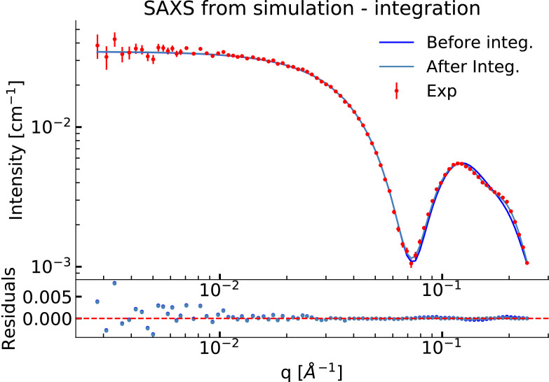
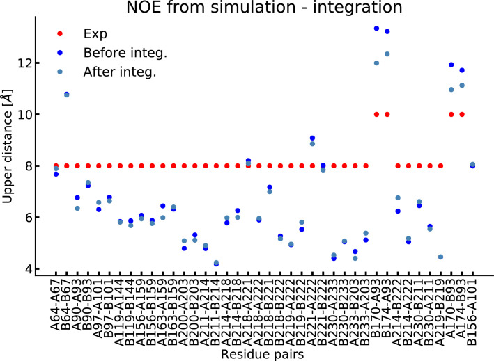
(A) SAXS data calculated from the simulation before and after reweighting the ensemble using experimental data. Only the high q-range is shown as the discrepancy between simulation and experiments are mainly located here (for the entire q-range see Figure 3—figure supplement 1). Agreement with the NOEs before and after integration are likewise shown in Figure 3—figure supplement 2. (B). Histogram of the acylindricity of the simulations ($\sqrt{C}$) both before integration (dark blue) and after integration (light blue). (C) Visualization of the conformational ensemble showing structures sampled every 100 ns in cartoon representation (blue), the original NMR/EPR structure is shown in rope representation for comparison (red). The table below shows the acylindricity of the entire conformational ensemble before and after integration and compared to the original NMR/EPR (NMR) structure and the SAXS/SANS model fit. (D) Weights and acylindricity of the three main clusters of the MD simulation (blue) before and after integration.

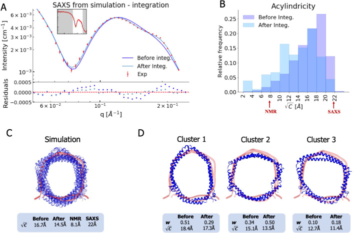
Figure 3—figure supplement 1. Comparison of the experimental SAXS data from simulation before and after integration.

This figure is an expanded version of that in the main text and shows agreement with the simulation after reweighting. SAXS data were calculated using FOXS.

Figure 3—figure supplement 2. NOEs from simulation before and after reweighting.

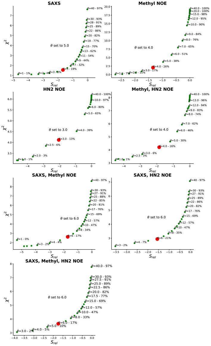
Figure 3—figure supplement 3. Determination of θ.

θ is a hyperparameter that tunes the balance between fitting the data accurately (low ${\mathrm{\chi }}_{\mathrm{r}}^{\mathrm{2}}$) and not deviating too much from the prior (low ${\mathrm{S}}_{\mathrm{\text{rel}}}$) thereby avoiding overfitting. It is here determined by plotting ${\mathrm{S}}_{\mathrm{\text{rel}}}$ vs ${\mathrm{\chi }}_{\mathrm{r}}^{\mathrm{2}}$ and selecting a value of θ near the natural kink and at a step where a similar decrease in ${\mathrm{\chi }}_{\mathrm{r}}^{\mathrm{2}}$ gives rise to a much lower ${\mathrm{S}}_{\mathrm{\text{rel}}}$, indicating that we cannot fit the to the experiments further without a risk of overfitting. The value of θ that produce the given (${\mathrm{S}}_{\mathrm{\text{rel}}}$,${\mathrm{\chi }}_{\mathrm{r}}^{\mathrm{2}}$) is annotated above the given point together with a measure of the effective number of frames used from the original simulation this gives rise to. Red dot marks the chosen θ.

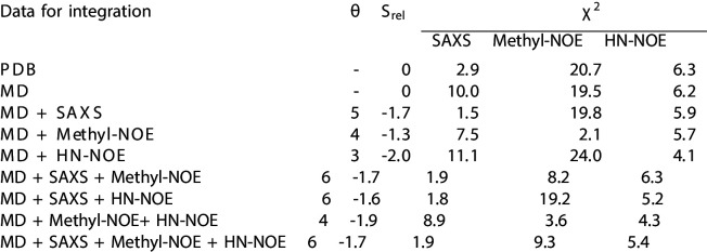
Figure 3—figure supplement 4. Combining experiments and simulations.

Similar analysis to the main text, but with the methyl- and HN-NOEs integrated individually. As can be seen, the methyl-NOE distances have a larger impact, likely due to the longer distances measured in methyl-NOE whereas the HN-NOEs mainly report on distances between atom pairs of 4 residues or less apart in the sequences and, thus, likely mainly on the helical secondary structure.