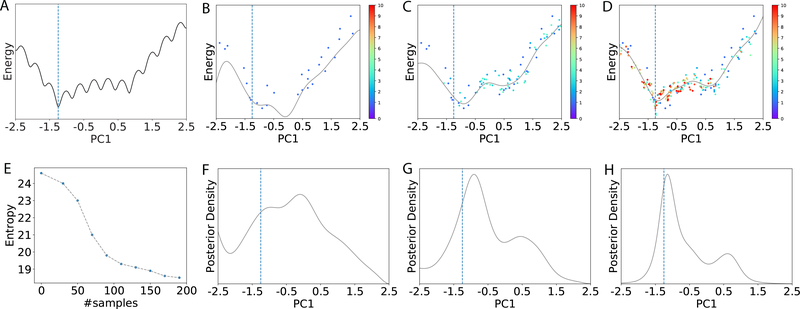
Figure 1:
Illustration of the Bayesian active learning (BAL) algorithm. (A): A typical energy landscape projected onto the first principal component (PC1) just for visualization, using all samples collected. The dashed line indicates the location of the optimal solution. (B)-(D): The samples (dots) and the kriging regressors (light curves) in the 1st, 4th and 10th iteration, respectively. Samples are colored from cold to hot for increasing iteration indices and those in the same iteration have the same color. (E): The entropy (measuring uncertainty) of the posterior reduces as the number of samples increases. Its quick drop, as the number of samples increases from 30 to 100, corresponds to a drastic change of the kriging regressor, which suggests increasing exploitation in possible function basins. After 100 samples, the entropy goes down more slowly, echoing the smaller updates of the regressor. (F)-(H): The corresponding posterior distributions for (B)-(D), respectively.

