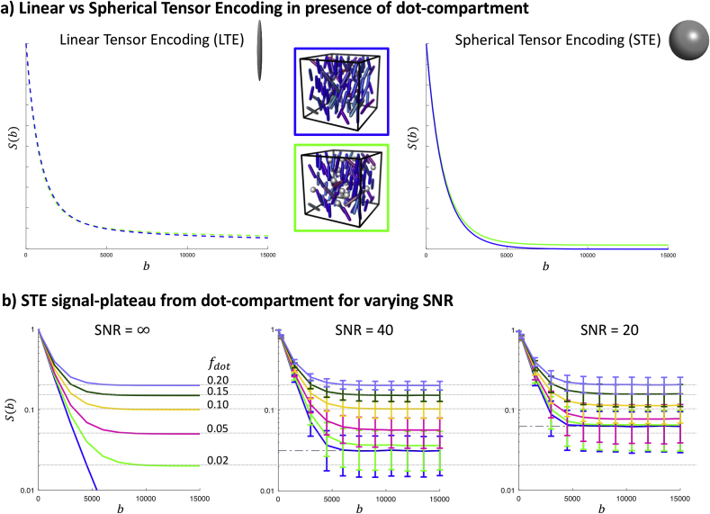
Fig. 1.

a) Simulations of LTE and STE data for two different scenarios (schematically represented in the middle): dispersed sticks representing axons surrounded by extra-axonal space (top, blue surround), vs dots ​+ ​dispersed sticks surrounded by extra-axonal space (bottom, green surround). Here, we used a Watson distribution to simulate a stick orientation dispersion (OD) of 0.7 and $f_{dot}=0$ (blue), and OD ​= ​0.5 and $f_{dot}=0.02$ (green). In both simulations, the parallel diffusivity was set to 2.1 ${\mathrm{\mu m}}^2/\mathrm{ms}$ for the stick compartment, and the extra-cellular compartment consisted of non-exchanging Watson-distributed ‘zeppelins’ with the same OD as the sticks and parallel and perpendicular diffusivities of 1.9 and 0.8 ${\mathrm{\mu m}}^2/\mathrm{ms}$, respectively. The two scenarios result in very similar signals for LTE across a wide b-value range, and can be disentangled better at high b-values with STE. A linear y-scale is chosen here to not make small differences seem disproportionally large. b) STE simulated as in (a) but with varying $f_{dot}$, at different SNR levels. The dashed-dotted line represents the rectified noise floor, and the error bars represent the mean and standard deviation over 5000 noise realisations. A logarithmic y-scale is chosen here to improve the visualisation for different $f_{dot}$. b is given in ${\text{s}/\text{mm}}^2$.