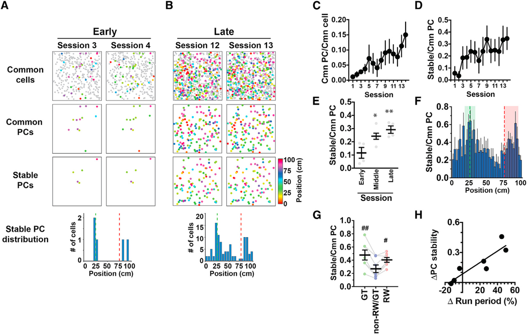
Figure 3. RW Cells and GT Cells Form Stable Singularities in Hippocampal Cognitive Maps.
(A) Example hippocampal CA1 PC maps imaged in two consecutive sessions in the early phase of the training. Maps shown on top, middle, and bottom present cells identified in common to both sessions (common cells), cells identified as PCs in both sessions (common PCs), and cells identified as PCs with stable (< 10 cm difference) place fields in both sessions (stable PCs), respectively. The histogram shown at the bottom indicates the distributions of the stable PCs against track position.
(B) PC maps imaged in the late phase of training in the same animal as presented in (A).
(C) The fraction of common PCs relative to the number of common cells identified in the two consecutive sessions that were compared. The x axis indicates the earlier of the two sessions that were compared. n = 7 mice.
(D) PC stability calculated as the fraction of stable PCs relative to the number of common PCs identified in the two consecutive sessions that were compared.
(E) Average PC stability in the early (sessions 1–4, numbered according to the earlier of the two sessions that were compared), middle (sessions 5–10), and late (sessions 11–14) phases of training. *p = 0.021 versus early, **p = 0.0050 versus early, F(2,11) = 8.04, one-way ANOVA; n = 4, 6, and 4 session pairs for the early, middle, and late phases, respectively.
(F) The average fractions of stable PCs relative to the number of common PCs plotted against track position. Values were calculated from data across all sessions and averaged for seven mice. The fractions were determined using the number of common PCs obtained separately for each spatial bin in the earlier of the two sessions compared. The green and red dashed lines delineate the positions of the landmark and reward delivery, respectively. The areas shown in green and red are those that define GT cells and RW cells, respectively.
(G) The average PC stability for GT, non-RW/GT, and RW cells. #p = 0.015 versus non-RW/GT cells, ##p = 0.0025 versus non-RW/GT cells, F(1.215,7.290) = 11.6, one-way ANOVA, n = 7 mice.
(H) The relationship between PC stability and learning to run along the track. The x axis presents the task performance of each mouse measured by the difference in the fraction of time spent running between the early (average of sessions 1–5) and late (average of sessions 11–15) phases of the training. The y axis presents the difference in PC stability between the early and late phases of training.
(C–G) Data are expressed as mean ± SEM.

