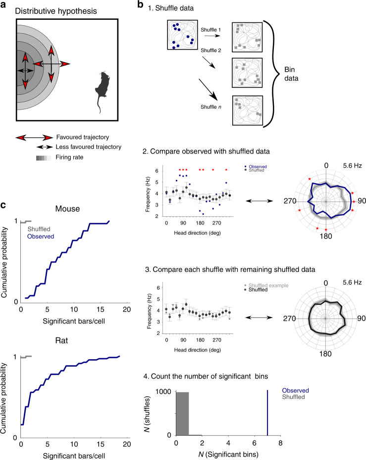
Fig. 2. The distributive hypothesis does not account for directional modulation.

a Schematic of directional tuning caused by behavioural bias that can be explained by the distributive hypothesis¹⁸. Red arrows indicate head directions likely to be more sampled relative to the directions indicated by the black arrows. Differences in sampling directions at the centre and edge of the field can lead to an apparent directional bias (Mouse schematic from scidraw.io (10.5281/zenodo.3910057, https://creativecommons.org/licenses/by/4.0/). b (1) Shuffled spike locations were generated by allocating spikes to the trajectory according to probabilities determined by the spatial firing rate map. Circles represent recorded spikes and squares represent shuffled spikes. (2) Observed and shuffled spike rates binned by head direction (bin width 18°, distributive plot) and visualized either with Cartesian (left) or polar coordinates (right). Error bars/shaded areas indicate the 90% confidence intervals of the shuffled data and the measure of centre is the mean. Asterisks indicate bins in which the observed data differs significantly from the shuffled data (p < 0.05, two-tailed p value calculated from the shuffled distribution and corrected for multiple comparisons with the Benjamini–Hochberg procedure). (3) As for step 2 but comparing individual shuffles to the overall shuffled distribution. (4) The number of significant bins in the observed data (determined as in step 2) and the shuffled data (determined by repeating step 3 for all shuffles). The example data are from the cell in Fig. 1b. c The distributions of the number of significant bins per cell differed significantly between observed and shuffled data (n = 34 grid cells from mice, p = 6.5 × 10⁻²⁴, U = 10.08; n = 68 grid cells from rats, p = 2.4 × 10⁻²⁹, U = 11.25, two-sided Mann–Whitney U test).