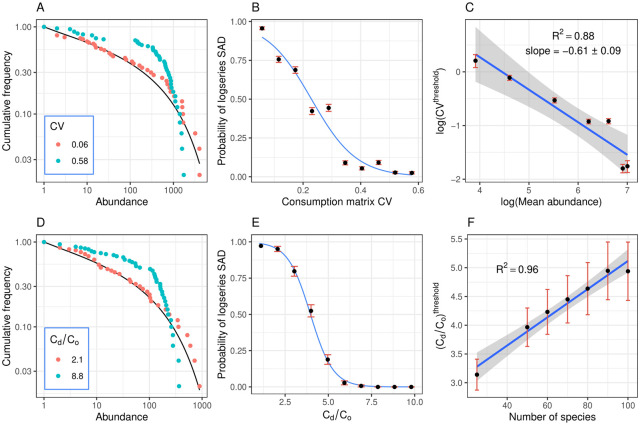
Fig 2. SAD results.

Species abundance distribution (SAD) results for the generalists scenarios (A-C) and specialist scenarios (D-F). A: In the generalist scenario, the log-series distribution (black curve) fits the SAD when the coefficient of variation (CV) in the consumption matrix is sufficiently low (red points; Cramér-von Mises goodness-of-fit test p-value 0.78), but is rejected when the CV is sufficiently high (blue points; CvM test p-value 0.02). B: Probability that the logs-series distribution fits the SAD decreases with the CV of the consumption matrix. Points and error bars show the mean and standard error of the count of successful fits, out of an ensemble of 106 communities. Blue curve shows logistic regression. The threshold CV, defined as the point where the probability falls below 50%, is CV^threshold = 0.23. C: log(CV^threshold) has a linear relationship with log(n), with slope −0.61 ± 0.09. This indicates a power law between CV^threshold and n, with an exponent close to our analytic prediction of −0.5. Error bars show uncertainty propagated from the standard errors of the fitted parameters in the respective logistic regressions. Bands show the 95% CI of the linear regression. D: In the specialists scenario, communities with low C_d/C_o ratio (red points; CvM test p-value 0.267) conform to the log-series distribution, while communities with sufficiently high C_d/C_o (blue points; CvM test p-value <0.001) reject the LS distribution. E: The probability of the LS distribution fitting the SAD decreases as C_d/C_o increases, with the threshold at $C_d^{\text{threshold}}=4.0$ (we set C_o = 1). Each data point summarizes an ensemble of 143 communities. F: $C_d^{\text{threshold}}$ increases linearly with the number of species in the community, in qualitative agreement with Eq 4. Parameters: A-B: K = S = 50, n = 500, r = 100. C: K = S = 50, r = 100. D-F: K = S = 50, n = r = 100.