Anatomical Context Protects Deep Learning from Adversarial Perturbations in Medical Imaging

Abstract

Deep learning has achieved impressive performance across a variety of tasks, including medical image processing. However, recent research has shown that deep neural networks are susceptible to small adversarial perturbations in the image. We study the impact of such adversarial perturbations in medical image processing where the goal is to predict an individual’s age based on a 3D MRI brain image. We consider two models: a conventional deep neural network, and a hybrid deep learning model which additionally uses features informed by anatomical context. We find that we can introduce significant errors in predicted age by adding imperceptible noise to an image, can accomplish this even for large batches of images using a single perturbation, and that the hybrid model is much more robust to adversarial perturbations than the conventional deep neural network. Our work highlights limitations of current deep learning techniques in clinical applications, and suggests a path forward.

1. Introduction

Deep learning methods are transforming the way scientists approach data across many disciplines, and have recently become prominent in medical imaging. For example, Esteva et al. [1] showed the same accuracy as a dermatologist in the detection of malignant skin lesions using deep learning techniques. Gulshan et al. [2] used similar methods for the detection of diabetic retinopathy in retinal fundus photographs with great accuracy, while Bejnordi et al. [3] were able to accurately detect lymph node metastasis in patients with breast cancer, and Cole et al. [4] used deep learning to produce a more accurate brain age prediction, which has been shown to correlate with neurodegenerative diseases. Given the remarkable results that deep learning methods have shown compared to standard clinical practice, these have started to be implemented into clinical practice, with several deep learning applications already approved by the United States Food and Drug Administration (FDA) [5, 6, 7, 8].

However, concerns regarding the clinical suitability / safety of deep learning models linger given their algorithmic complexity and difficulty in describing specifically which features are driving the models. The lack of clarity may mask the true image content being learned (e.g., the difference between a wolf and a dog might be that wolves are seen in the snow [9]) or conceal issues of fairness [10]. Additionally, potential deleterious consequences of the opacity of deep learning have recently come to the fore in the computer vision community (largely, focusing on image classification tasks), where several studies reveal vulnerability of deep learning models to unanticipated perturbations, commonly known as adversarial examples [11, 12, 13, 14, 15, 16]. In particular, a number of methods have emerged which make small modifications to images that are indistinguishable to human eye, but effect dramatically different predictions. Similar observations have recently been made in the field of medical imaging for several classification and segmentation tasks [17, 18, 19], raising the concern that either faulty medical imaging equipment, or even unscrupulous for-profit providers, would lead to diagnostic mistakes (for example, leading to unnecessary additional testing).

We present the first investigation of vulnerabilities of regression-based prediction in medical image processing to adversarial example attacks. Specifically, our problem setting involves predicting age of a subject based on their 3D MRI brain image, with malicious perturbations artificially injected directly into the digital images. Since prior adversarial example research is focused on classification or segmentation tasks, our first contribution is to adapt state-of-the-art methods for generating adversarial examples with l₀, l₂, and l_∞ constraints on the magnitude of the perturbation to our setting. Our second contribution is a method for generating universal adversarial perturbations for our domain—that is, a single perturbations (for each norm) that is effective on a large batch of images; this is entirely novel in the context of medical imaging. Our third contribution is to experimentally demonstrate that adversarial examples—both image-specific, and universal—are indeed extremely effective, significantly reducing prediction effectiveness of deep learning for age prediction. The observation of the effectiveness of universal perturbations in this setting is particularly powerful: it implies that a single malfunction in MRI equipment (inadvertent, or adversarial) can have a significant impact.

Given vulnerability of deep learning for medical imaging, it is natural to wonder whether one can effectively mitigate this issue. We explore one approach which has not previously been considered for this: augmenting deep learning models with volumetric features obtained through traditional multi-atlas segmentation techniques, where each feature corresponds to the volume of a brain region (for a total of 132 features). Such contextual information has previously been shown effective in improving prediction in non-adversarial settings [20, 21, 22], and is by construction relatively insensitive to small perturbations. Our forth contribution is to demonstrate experimentally that, indeed, adding contextual features to deep learning significantly mitigates its vulnerability to adversarial perturbations, whether they are designed for each image independently, or universally crafted for batches of images.

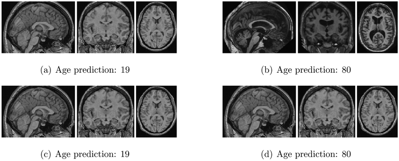
To illustrate the effect of adversarial noise, consider Figure 1, where age is predicted using a conventional deep neural network. For this figure, we identify one sample with predicted age 19 and another sample with predicted age 80 (Figures 1(a) and 1(b), respectively); we note that predictions on unperturbed data are extremely accurate (root mean squared error, RMSE < 5.13 years). Comparing the brain images of a 19 and 80 year-old, we can readily see clear differences between them. Next, we add low-magnitude random noise (l_∞ of noise is 0.002, where pixel values are normalized between 0 and 1) to the first (19-year-old) sample (Figure 1(c)), showing that the deep neural network is robust to such random perturbations. Figure 1(d) contrasts this with an adversarial perturbation of the same magnitude, but which causes the neural network to predict that the subject’s age is 80!

Figure 1:

The illustration of the effect of adversarial attack. (a) Sample 1 (19 year-old). (b) Sample 2 (80 year-old). (c) Sample 1 with random noise. (d) Sample 1 with adversarial perturbation. The difference among (a), (c) and (d) appears imperceptible to human eye.

2. Methods

First, we describe the approaches we used to generate adversarial perturbations for a single image. Subsequently, we present our approach that targets a batch of images with a single perturbation. All our code is publicly available at https://github.com/yvorobey/adversarialMI.

2.1. Generating Adversarial Perturbations for a Single Image

Let F(x) be the function computed by the deep neural network to predict age for an arbitrary input image x. Consider a fixed image x₀. Our goal is to generate a small (imperceptible) perturbation, Δx, to add to the original image x₀, so as to maximize or minimize predicted age. As described earlier, we use l_∞, l₂, and l₀ norms to quantify the magnitude of the introduced perturbation. In all cases, if we wish to maximize predicted age, the goal is to solve the following problem:

$$\begin{gathered} {\text{maximize}}_{\Delta x}G(\Delta x)=F(x_0+\Delta x) \\ \text{subject}\text{to}:\Vert \Delta x{\Vert }_p\le ϵ,x_0+\Delta x\in [0,1{]}^n \end{gathered}$$ (1)

where ∥ · ∥_p corresponds to the one of the above norms (p = ∞, 2, and 0, respectively), F(x + Δx) is the predicted age for the perturbed image, and the constraint ∥Δx∥_p ≤ ϵ ensures that perturbation is at most ϵ, which is a small and exogenously specified bound (in our experiments, at most 0.002 for any norm). Additionally, since image pixels are normalized in the [0, 1] interval, we also ensure that introduced perturbations result in valid images by adding the constraint that x₀+Δx ∈ [0, 1]ⁿ. If our goal is to minimize, rather than maximize predicted age, the objective becomes minimization rather than maximization.

Since the optimization problem (1) is challenging as stated, we use heuristic approaches based on those introduced in prior literature for solving this problem [11]. As the specific approaches are tailored to the norm which measures the magnitude of the introduced perturbation, we next present such approaches for each norm.

2.1.1. The l_∞ Attack

Our approach to implementing the l_∞ norm attack is based on FGSM [12] and its subsequent iterative variation [28]. The idea behind the approach is to approximate the objective function F(x₀ + Δx) ≈ ∇F(x₀)Δx + F(x₀). The optimal solution to this linearized objective is then Δx = ϵ sign(∇F(x₀)). Extending this idea to an iterative variant, with N the number of iterations, we can take steps of size ϵ/N, where each step computes Δx using the gradient sign approach starting from the previous iterate. Finally, if the total modification to x₀ ever leaves the interval [0, 1], it is clipped to remain feasible. The full algorithm is given in Algorithm 1.

Algorithm 1 Single Target l∞ Attack

$$\begin{array}{cc}\hfill & 1\mathbf{input}:\text{predictor}F,l_{\infty }\text{distance}ϵ,\text{iteration steps}N,\text{original image}{x}_0\hfill \\ \hfill & 2\mathbf{output}:\text{adversarial}\text{perturbation}\Delta x\hfill \\ \hfill & 3t\leftarrow 0,i\leftarrow 0\hfill \\ \hfill & 4\alpha \leftarrow ϵ∕N\hfill \\ \hfill & 5\mathbf{while}i<N:\hfill \\ \hfill & 6t\leftarrow t+\alpha \cdot \text{sign}(\nabla F(x_0+t))\hfill \\ \hfill & 7t\leftarrow {\text{clip}}_{[0,1]}(x_0+t)\hfill \\ \hfill & 8i\leftarrow i+1\hfill \\ \hfill & 9\Delta x\leftarrow t\hfill \end{array}$$

In the algorithm, the statement t ← clip_[0,1](x₀ + t) clips the argument to stay in the [0, 1] interval, modifying t accordingly.

These ideas extend in a straightforward way to minimizing F(x₀ + Δx).

2.1.2. The l₂ Attack

Our approach for generating adversarial perturbations with respect to the l₂ norm follows Szegedy et al. [14] and Carlini and Wagner [16].

The main idea is to replace the hard constraint that ∥δx∥₂ ≤ ϵ with an associated penalty in the objective. Specifically, we rewrite Problem (1) as follows:

$$\begin{gathered} {\text{minimize}}_{\Delta x}-c\cdot F(x_0+\Delta x)+\Vert \Delta x{\Vert }_2 \\ \text{subject}\text{to}:x_0+\Delta x\in [0,1{]}^n \end{gathered}$$ (2)

The constant c is used to balance maximizing F(x+Δx) and minimizing ∥Δx∥₂. By updating c, we can then find a Δx which satisfies ∥Δx∥₂ ≤ ϵ and maximizes F(x + Δx).

To deal with the box constraint 0 ≤ x₀ + Δx ≤ 1, we follow Carlini and Wagner [16] and apply a change-of-variables, introducing a new variable ω such that:

$$\begin{gathered} x_0=\frac{1}{2}(\tanh ({\omega }_0)+1) \\ \Delta x=\frac{1}{2}(\tanh ({\omega }_0+\Delta \omega )-\tanh ({\omega }_0)) \end{gathered}$$

Since −1 ≤ tanh(ω) ≤ 1, the constraint 0 ≤ x₀ + Δx ≤ 1 is always satisfied. With this transformation, we optimize over ω, rather than Δx. The transformed optimization problem becomes

$${\text{minimize}}_{\Delta \omega }-c\cdot F\left(\frac{1}{2}(\tanh ({\omega }_0+\Delta \omega )+1)\right)+\Vert \tanh ({\omega }_0+\Delta \omega )-\tanh ({\omega }_0){\Vert }_2.$$

The algorithm is shown as in Algorithm 2. In this algorithm, the optimizer uses N steps to find the optimal solution with the specific constant c. Every time we run the optimizer, it would try to make the result of −c · F(x₀ + Δx) + ∥Δx∥₂ smaller at a certain learning rate. After each time we run the optimizer, we would check whether the l₂ distance is smaller than the ϵ we have set and compare F(x₀ + Δx) with the current maximum result.

Algorithm 2 Single Target l2 Attack

$$\begin{array}{cc}\hfill & 1\mathbf{input}:\text{image}{x}_0,\text{predictor}F,L_2\text{distance}ϵ,\text{number}\text{of}\text{iterations}N,\text{number}\text{of}\hfill \\ \hfill & \text{iterations}\text{of}\text{binary}\text{search}m\hfill \\ \hfill & 2\mathbf{output}:\text{adversarial}\text{perturbation}\Delta x\hfill \\ \hfill & 3\text{initialize}{x}^{\prime }\leftarrow x,c\leftarrow c_0,i\leftarrow 0\hfill \\ \hfill & 4{\omega }_0\leftarrow {\tanh }^{-1}(2x-1)\hfill \\ \hfill & 5\mathbf{while}i<m\hfill \\ \hfill & 6\text{flag}\leftarrow \text{False}\hfill \\ \hfill & 7\text{optimizer}\leftarrow \text{optimizer}.\text{minimize}(-c\cdot F\left(\frac{1}{2}(\tanh ({\omega }_0+\Delta \omega )+1)\right)+\Vert \tanh ({\omega }_0+\Delta \omega )-\tanh ({\omega }_0){\Vert }_2)\hfill \\ \hfill & 8\mathbf{while}j<N:\hfill \\ \hfill & 9\Delta \omega \leftarrow \text{optimizer}.\text{run}\_\text{one}\_\text{step}\hfill \\ \hfill & 10\Delta x\leftarrow \frac{1}{2}(\tanh ({\omega }_0+\Delta \omega )-\tanh ({\omega }_0))\hfill \\ \hfill & 11\mathbf{if}\Vert \Delta x{\Vert }_2<ϵ:\hfill \\ \hfill & 12\text{flag}\leftarrow \text{True}\hfill \\ \hfill & 13\mathbf{if}F(x+\Delta x)>F(x^{\prime }):\hfill \\ \hfill & 14x^{\prime }\leftarrow x+\Delta x\hfill \\ \hfill & 15j\leftarrow j+1\hfill \\ \hfill & 16\mathbf{if}\text{flag}:\hfill \\ \hfill & 17\text{increase}c\hfill \\ \hfill & 18\mathbf{else}\hfill \\ \hfill & 19\text{decrease}c\hfill \\ \hfill & 20i\leftarrow i+1\hfill \\ \hfill & 21\Delta x\leftarrow x^{\prime }-x_0\hfill \end{array}$$

As before, the approach is straightforward to modify if we wish to minimize predicted age.

2.1.3. The l₀ attack

In the l₀ attack, the goal is to introduce an adversarial perturbation by modifying fewer than ϵ pixels in the image. Our method for doing this uses the intuition that the pixels with higher absolute gradient value play a more important role in the prediction output. Consequently, we find the pixels with the maximum absolute value of the gradient, and try to modify the value of these to maximize or minimize the model prediction. We iteratively do this until the maximum l₀ distance is achieved (i.e., we reach the threshold number of pixels we can modify). This approach for maximizing the prediction is formalized in Algorithm 3. To minimize predicted age, the only difference is to modify the value of one pixel in each iteration to make the prediction smaller, rather than larger.

Algorithm 3 Single Target l0 Attack

$$\begin{array}{cc}\hfill & 1\mathbf{input}:\text{image}{x}_0,\text{predictor}F,l_0\text{distance}\text{upper}\text{bound}ϵ,\text{possible}\text{values}\text{for}\text{each}\text{pixel}\hfill \\ \hfill & V=[v_1,v_2,\dots v_n]\hfill \\ \hfill & 2\mathbf{output}:\text{adversarial}\text{perturbation}\Delta x\hfill \\ \hfill & 3\text{initialize}{x}^{\prime }\leftarrow x_0,i\leftarrow 0\hfill \\ \hfill & 4G\leftarrow {\nabla }_{x}F(x^{\prime })\hfill \\ \hfill & 5\mathbf{while}i<ϵ:\hfill \\ \hfill & 6pos\leftarrow argma{x}_k(\mid G_k\mid )\hfill \\ \hfill & 7G_{pos}\leftarrow 0\hfill \\ \hfill & 8flag\leftarrow False\hfill \\ \hfill & 9\mathbf{for}k\mathbf{in}V:\hfill \\ \hfill & 10x^{″}\leftarrow x^{\prime }\hfill \\ \hfill & 11x_{pos}^{″}\leftarrow k\hfill \\ \hfill & 12\mathbf{if}f(x^{″})>f(x^{\prime }):\hfill \\ \hfill & 13x^{\prime }\leftarrow x^{″}\hfill \\ \hfill & 14flag\leftarrow True\hfill \\ \hfill & 15\mathbf{if}\text{flag}:\hfill \\ \hfill & 16i\leftarrow i+1∕size(x)\hfill \\ \hfill & 17\Delta x\leftarrow x^{\prime }-x_0\hfill \end{array}$$

2.2. Generating Adversarial Perturbations for a Batch of Images

Our final discussion concerns a method for generating a single adversarial perturbation Δx for a batch of input images {x₀, x₁, …, x_m}. We formalize it as solving the following optimization problem:

$$\begin{gathered} \text{Maximize}G(\Delta x)=\sum _{i=0}^{m}F(x_i+\Delta x) \\ \text{subject}\text{to}:\Vert \Delta x{\Vert }_{\infty }\le ϵ \end{gathered}$$ (3)

(Note that we restrict attention to l_∞-norm attacks in this case, to simplify discussion.)

We optimize the objective by extending the iterative gradient-sign method discussed in Section 2.1.3. The full algorithm is given in Algorithm 4.

Algorithm 4 l∞ Attack for a batch of images

$$\begin{array}{cc}\hfill & 1\mathbf{input}:\text{a batch}\text{of}\text{original}\text{images}\{x_0,x_1,\dots ,x_m\},\text{predictor}F,l_{\infty }\text{upper bound}ϵ,\text{number}\hfill \\ \hfill & \mathsf{o}\mathsf{f}\text{iterations}N\hfill \\ \hfill & 2\mathbf{output}:\text{adversarial}\text{perturbation}\Delta x\hfill \\ \hfill & 3t\leftarrow 0,j\leftarrow 0\hfill \\ \hfill & 4\alpha \leftarrow ϵ∕N\hfill \\ \hfill & 5\mathbf{while}j<N:\hfill \\ \hfill & 6t\leftarrow t+\alpha \cdot \text{sign}\left(\sum _{i=0}^m\nabla F(x_i+t)\right)\hfill \\ \hfill & 7j\leftarrow j+1\hfill \\ \hfill & 8\Delta x\leftarrow t\hfill \end{array}$$

3. Results

Here we focus on data that are generally accessible and with an algorithm not likely to drive patient care to evaluate the effectiveness of such attacks in medical image processing settings in a way that does not violate clinical research ethics (as could be an issue, for example, if the target was a medical diagnosis). We expect that our results are generalizable, so long as similar image processing techniques are used.

Our imaging dataset is an aggregate of 7 datasets with a total 3921 T1w 3D images from normal, healthy subjects. The data include subjects with ages ranging between 4 and 94 years old, with a mean age and standard deviation of 25.5 ± 18.6 years. Of the 3921 subjects, 54.2% were male and 45.8% were female. Data were also acquired from different sites so there is a difference in field strength, of which 71.5% of scans were acquired at 3 Tesla and 28.5% were acquired at 1.5 Tesla. ROI volumes, gender, and field strength were all used as input features for age prediction.

We consider two models for predicting age: 1) a conventional deep neural network, and 2) a hybrid (or context-aware) model which combines deep learning with image segmentation techniques. The conventional deep neural network model (Conventional DNN) takes a 3D brain MRI image as input and produces a subject’s age as output. The architecture consists of five 3D convolution layers of increasing size followed by two densely connected layers and one output layer. The ReLU activation function was used for all hidden layers. The neural network was trained using a learning rate of 0.001. The structure of this model is shown in Figure 2(a). The context-aware model has a similar structure to the conventional deep neural network model, with the exception that 132 volumetric features are introduced after the convolutional layers followed by two densely connected layers and, finally, the output layer. Volumetric estimates for 132 regions of interest in the brain (that is, each feature corresponds to the volume of a region of interest) were obtained using multi-atlas segmentation [23, 24]. The structure of the context-aware model is demonstrated in Figure 2(b).

Figure 2:

The models for brain age prediction

We consider three types of attacks which inject adversarial noise into an image: l_∞ attack, l₀ attack, and l₂ attack. All attacks limit the amount of noise being injected to ensure that is cannot be perceived by looking at the image, but differ in how they measure the amount of noise injected. The l_∞ attack considers modification to each pixel independently, and limits the amount any pixel can be modified. The l₀ attack limits the number of pixels modified. The l₂ attack limits the Euclidean norm of the injected adversarial perturbation. More precisely, define the perturbation as Δx = (Δx₀, …, Δx_N), where N is the number of pixels in the image. We define distortions in the respective norms as follows (we use slightly modified definitions here to make our results more intuitive):

$$l_{\infty }:\underset{i=0}{\overset{N}{\max }}\{\Delta x_i\},l_2:\sqrt{\frac{1}{N}\sum _{i=0}^N\Delta x_i^2},l_0:\frac{1}{N}\sum _{i=0}^{N}1(\Delta x_i\ne 0).$$ (4)

The value of pixels in the original samples was normalized into range [0, 1].

The goal of adversarial perturbations is to either maximize or minimize the predicted (as opposed to actual) age. Since original predictions (without adversarial noise) are quite good (RMSE < 5.13 years), we use those as a baseline. We then measure the effectiveness of adversarial noise (in skewing the predictions) by deviation, defined as absolute change in predicted age:

$$\mathit{deviation}=\mid y^{\prime }-y\mid ,$$ (5)

where y is the original prediction (without noise), and y′ the prediction after adversarial perturbation.

3.1. Conventional Deep Neural Networks are Fragile to Adversarial Perturbations of Medical Images

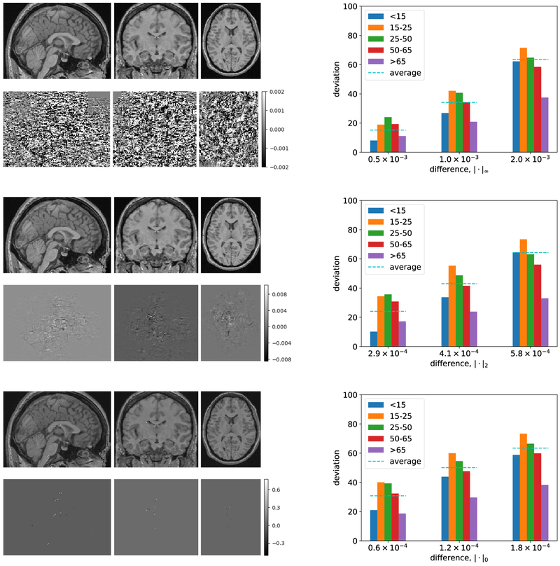
We first consider the impact of adversarial perturbations on a Conventional DNN, where we aim to maximize predicted age. Figure 3 illustrates this for the 19-year-old subject we discussed earlier, and presents results over the entire dataset, breaking these down by (originally predicted) age groups: 0–14, 15–25, 26–50, 51–65, and > 65. As we can see from the illustration (images in the left column of the figure), we can cause the conventional DNN to predict age as 80 (rather than 19) using any of the three ways to quantify perturbation, with all three brain images looking indistinguishable from the original (in Figure 1(a)). As we would anticipate, l₀ perturbations are the most sparse, concentrated in parts of the image that have the greatest impact. A more systematic analysis in Figure 3 (plots in the right column) shows that age can be amplified nearly 70 years on average by adding perturbation with magnitude < 0.002 (for the normalized image) by any of the three measures. Interestingly, the most susceptible population is 15-25 year olds, across all three attack methods.

Figure 3:

The adversarial perturbations that aim to maximize age. Images in the left column display the results of adversarial perturbations to the image of a 19-year-old subject in Figure 1(a), using each of our three criteria for limiting the magnitude of the perturbation. The images in the top row of each of these correspond to the modified 2D slice images of the brain; immediately below is isolated noise that we add (amplified for visibility). In the right column we present general results of applying adversarial perturbations to images in our data (maximizing predicted age). In each plot, the x-axis is the limit of the amount of noise injected (where the noise bound is measured by each of our three l_p measures), while the y-axis is the corresponding impact, measured by deviation from original prediction. The first row of plots correspond to l_∞-bounded perturbations. The second row of plots represent results for l₂-bounded perturbations. The third row of plots are the results for l₀-bounded perturbations.

Similar trends are obtained if we inject adversarial noise in order to minimize predicted age (Figure 4). There appears to be little difference in which metric we use to bound adversarial perturbations: in all cases, with only a small amount of added noise, we can often reduce predicted age to nearly 0 for all age cohorts.

Figure 4:

Attacks that aim to minimize predicted age. The x-axis limits the amount of noise injected, while the y-axis shows the corresponding impact, measured by deviation from original prediction. Left: adversarial perturbations bounded by the l_∞ metric. Middle: adversarial perturbations bounded by the l₂ metric. Right: adversarial perturbations bounded by the l₀ metric.

3.2. A Single Adversarial Perturbation Works for Large Batches of Images

While the most powerful attacks customize adversarial noise to each image, an alternative that may be more practical is to generate a single perturbation which can then be injected into any given image. We design such an attack, based on the l_∞-norm framework (which bounds the most any one pixel can be changed), and investigate its effectiveness as a function of the number of images that we target with a single attack. The attack maximizes average predicted age for an entire batch of images.

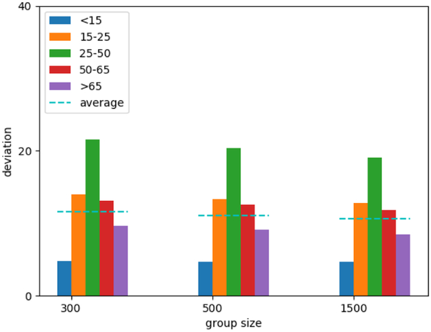
Figure 5 presents the results. Interestingly, once we consider more than 300 images in a batch, increasing the batch size has a relatively small impact on the effectiveness of adversarial perturbations. On average, perturbations result in an error in predicted of over 10 years (averaged over images in the batch, and random draws of batches), even when we consider batches of 1500 images. In the case of the most vulnerable cohort (<25-50 years old, in this case), the impact is over 20 years. Consequently, we can design highly effective adversarial perturbations that appear to be nearly universal.

Figure 5:

Attacking multiple images using the same adversarial perturbation for the conventional DNN model. The attack maximizes predicted age. We set the modification distance to 0.002. Group size corresponds to the number of images that we target with a single adversarial perturbation.

3.3. Deep Learning with Volumetric Features based on Image Segmentation is Less Vulnerable

One of our most significant observations is not just that the conventional DNN model is vulnerable, but that incorporating features based on traditional multi-atlas image segmentation makes it significantly less vulnerable to adversarial perturbations.

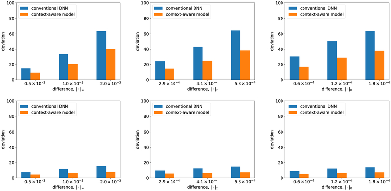
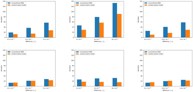
Consider Figure 6 which presents the systematic analysis of the impact of adversarial perturbations on the context-aware model.¹ The difference with the conventional DNN is evident: in every case, the impact of the attack is significantly reduced, often by several factored. Nevertheless, it is not eliminated. For example, we can still introduce imperceptible noise (changing pixels by at most 0.2%) and in many cases increase predicted age by over 30 years.

Figure 6:

Adversarial perturbations designed for the context-aware model. The x-axis limits the amount of noise injected, while the y-axis shows the corresponding impact, measured by deviation from original prediction. Left plots correspond to l_∞ bounds (the most any one pixel can be changed) to measure impact. Middle plots correspond to l₂ bounds (Euclidean norm of the added noise). Right plots correspond to l₀ bounds (the fraction of pixels that can be changed). Top plots correspond to the objective of maximizing predicted age. Bottom plots are when we aim to minimize predicted age

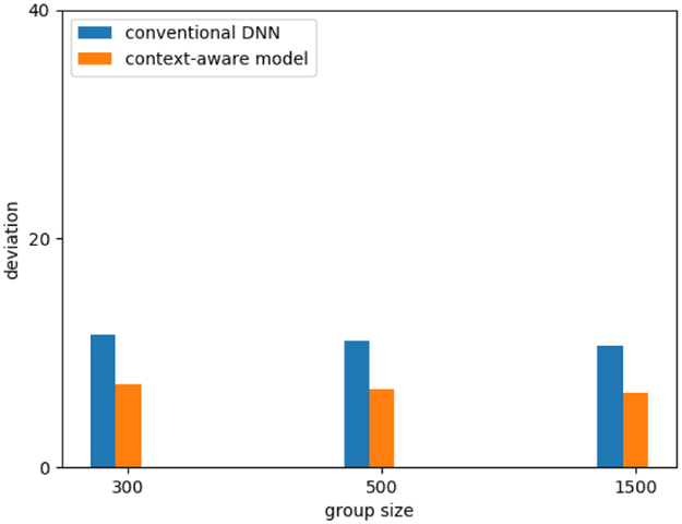
Similarly, we can observe that the impact of adversarial perturbations on image batches is significantly reduced for the context-aware model (Figure 7), where average impact on age drops from approximately 10 to just over 5 years. This drop is especially noteworthy since the adversarially induced error is now similar to the RMSE of the model prior to adversarial perturbations (which is just over 5 years).

Figure 7:

Attacking multiple images using the same adversarial perturbation for the context-aware model. The attack maximizes predicted age. We set the modification distance to 0.002. Group size corresponds to the number of images that we target with a single adversarial perturbation.

4. Discussion

Despite the increasing popularity of deep learning methods in medical imaging applications, our results suggest that significant concerns remain about robustness of these to adversarial perturbations to the environment. Such perturbations may arise simply due to unanticipated use cases or unusual patients, but may also be a product of actual tampering, for example, aiming to exploit introduced diagnostic bias for economic gain. While DICOM supports robust security protocols, common software features are not uniformly implemented or applied [25], and data may be vulnerable to simple, direct manipulation on portable data systems (e.g., reliance on physical CD transport). While one may be skeptical about the practical relevance of adversarial perturbations to individual images, our results suggest that we can even generate a single perturbation which introduces significant bias into predictions made on many images. Moreover, the relatively opaque nature of deep learning models makes the problem particularly challenging, as erroneous predictions may be difficult to detect.

However, our results also suggest that a way to address fragility of deep learning models is by incorporating domain knowledge and more traditional multi-atlas image segmentation techniques. We believe that such methods introduce higher-level semantic information into the model which is significantly more robust to voxel-level image perturbations. While our experiments suggest that such a context-aware model may still be somewhat vulnerable to adversarial noise, it is significantly less so that a pure (conventional) deep neural network. Alternative approaches, such as adversarial retraining [26, 27], have also shown promise in significantly reducing vulnerability of machine learning algorithms, including deep learning, to adversarial perturbations. In the end, it is likely that a combination of techniques is needed to make deep learning sufficiently reliable for medical image processing applications.

Biography

Yi Li is a Ph.D student in the Department of Computer Science at Vanderbilt University under the mentorship of Yevgeniy Vorobeychik. His current research is focused on robust learning algorithms in Cyber-Physical Systems.

Huahong Zhang is a Ph.D. student in the Department of Computer Science at Vanderbilt University. His research interests include deep learning and image processing, with application to biomedical image synthesis and segmentation.

Yifan Chen is a senior student at Vanderbilt University majoring in Computer Science and Applied Mathematics. His research interest is on analyzing the properties of adversarial examples for neural networks. He also interned at Alibaba, a world-leading e-commerce company, and developed a CNN-based service that automatically generates advertisement page for online clothing stores.

Camilo Bermudez Noguera is an M.D. - Ph.D. student in the Department of Biomedical Engineering at Vanderbilt University under the mentorship of Bennett Landman, Ph.D. His current research is focused on the development and validation of quantitative biomarkers from clinical and imaging datasets to inform medical decision making.

Bennett Landman is currently an Associate Professor of Electrical Engineering at Vanderbilt University, with secondary appointments in Computer Science, Biomedical Engineering, Radiology and Radiological Sciences, and Psychiatry and Behavioral Sciences. His research concentrates on applying image-processing technologies to leverage large-scale imaging studies to improve understanding of individual anatomy and personalize medicine.

Yevgeniy Vorobeychik is currently an Associate Professor of Computer Science and Engineering at Washington University in St. Louis. His research focuses on adversarial machine learning, computational game theory, and network science.

Appendix A.

Since multi-atlas features regeneration takes too long, the results presented in Figure 6 do not consider the changes of multi-atlas feature after the attacks. Figure A.8 presents the results with regenerated multi-atlas feature on a tiny data set (8 instances). Although we can’t generate enough data to make any strong claims about the comparisons, but it’s enough evidence to suggest that, indeed, attacks don’t make a significant impact on the multi-atlas features.

Figure A.8:

Adversarial perturbations designed for the context-aware model with regenerated multi-atlas features. The x-axis limits the amount of noise injected, while the y-axis shows the corresponding impact, measured by deviation from original prediction. Left plots correspond to l_∞ bounds (the most any one pixel can be changed) to measure impact. Middle plots correspond to l₂ bounds (Euclidean norm of the added noise). Right plots correspond to l₀ bounds (the fraction of pixels that can be changed). Top plots correspond to the objective of maximizing predicted age. Bottom plots are when we aim to minimize predicted age

References

- [1].Esteva A, Kuprel B, Novoa RA, Ko J, Swetter SM, Blau HM, Thrun S, Dermatologist-level classification of skin cancer with deep neural networks, Nature 542 (7639) (2017) 115. [DOI] [PMC free article] [PubMed] [Google Scholar]
- [2].Gulshan V, Peng L, Coram M, Stumpe MC, Wu D, Narayanaswamy A, Venugopalan S, Widner K, Madams T, Cuadros J, et al. , Development and validation of a deep learning algorithm for detection of diabetic retinopathy in retinal fundus photographs, Journal of the American Medical Association 316 (22) (2016) 2402–2410. [DOI] [PubMed] [Google Scholar]
- [3].Bejnordi BE, Veta M, van Diest PJ, van Ginneken B, Karssemeijer N, Litjens G, van der Laak JA, Hermsen M, Manson QF, Balkenhol M, et al. , Diagnostic assessment of deep learning algorithms for detection of lymph node metastases in women with breast cancer, Journal of the American Medical Association 318 (22) (2017) 2199–2210. [DOI] [PMC free article] [PubMed] [Google Scholar]
- [4].Cole JH, Poudel RP, Tsagkrasoulis D, Caan MW, Steves C, Spector TD, Montana G, Predicting brain age with deep learning from raw imaging data results in a reliable and heritable biomarker, NeuroImage 163 (2017) 115–124. [DOI] [PubMed] [Google Scholar]
- [5].F.D.A. approval letter: Arterys software v2.0 (October 2016). URL https://www.accessdata.fda.gov/cdrh_docs/pdf16/K162513.pdf
- [6].F.D.A. approval letter: Butterfly network (September 2017). URL https://www.accessdata.fda.gov/cdrh_docs/pdf16/K163510.pdf
- [7].F.D.A. approval letter: Quantitative insights (May 2017). URL https://www.accessdata.fda.gov/cdrh_docs/pdf16/K163510.pdf
- [8].F.D.A. approval letter: Quantitative insights (March 2017). URL https://www.accessdata.fda.gov/cdrh_docs/pdf16/K162627.pdf
- [9].Ribeiro MT, Singh S, Guestrin C, “why should I trust you?”: Explaining the predictions of any classifier, CoRR abs/1602.04938. arXiv:1602.04938. URL http://arxiv.org/abs/1602.04938 [Google Scholar]
- [10].Burrell J, How the machine ‘thinks’: Understanding opacity in machine learning algorithms, Big Data & Society 3 (1) (2016) 2053951715622512. [Google Scholar]
- [11].Vorobeychik Y, Kantarcioglu M, Adversarial Machine Learning, Morgan and Claypool, 2018. [Google Scholar]
- [12].Goodfellow IJ, Shlens J, Szegedy C, Explaining and harnessing adversarial examples, in: International Conference on Learning Representations, 2015. [Google Scholar]
- [13].Kurakin A, Goodfellow IJ, Bengio S, Adversarial machine learning at scale, in: International Conference on Learning Representations, 2017. [Google Scholar]
- [14].Szegedy C, Zaremba W, Sutskever I, Bruna J, Erhan D, Goodfellow IJ, Fergus R, Intriguing properties of neural networks, in: International Conference on Learning Representations, 2013. [Google Scholar]
- [15].Nguyen A, Yosinski J, Clune J, Deep neural networks are easily fooled: High confidence predictions for unrecognizable images, in: IEEE Conference on Computer Vision and Pattern Recognition, 2015, pp. 427–436. [Google Scholar]
- [16].Carlini N, Wagner D, Towards evaluating the robustness of neural networks, in: IEEE Symposium on Security and Privacy, 2017, pp. 39–57. [Google Scholar]
- [17].Paschali M, Conjeti S, Navarro F, Navab N, Generalizability vs. robustness: investigating medical imaging networks using adversarial examples, in: International Conference on Medical Image Computing and Computer-Assisted Intervention, Springer, 2018, pp. 493–501. [Google Scholar]
- [18].Taghanaki SA, Das A, Hamarneh G, Vulnerability analysis of chest x-ray image classification against adversarial attacks, in: Understanding and Interpreting Machine Learning in Medical Image Computing Applications, Springer, 2018, pp. 87–94. [Google Scholar]
- [19].Finlayson SG, Kohane IS, Beam AL, Adversarial attacks against medical deep learning systems, arXiv preprint arXiv:1804.05296. [Google Scholar]
- [20].Bermudez C, Plassard AJ, Chaganti S, Huo Y, Aboud KE, Cutting LE, Resnick SM, and Landman BA, Anatomical context improves deep learning on the brain age estimation task, in: Magnetic Resonance Imaging 62 (2019) 70–77. [DOI] [PMC free article] [PubMed] [Google Scholar]
- [21].Kong B, Wang X, Li Z, Song Q, Zhang S, Cancer metastasis detection via spatially structured deep network, in: International Conference on Information Processing in Medical Imaging, Springer, 2017, pp. 236–248. [Google Scholar]
- [22].Yan Z, Zhan Y, Peng Z, Liao S, Shinagawa Y, Zhang S, Metaxas DN, Zhou XS, Multi-instance deep learning: Discover discriminative local anatomies for body-part recognition, IEEE transactions on medical imaging 35 (5) (2016) 1332–1343. [DOI] [PubMed] [Google Scholar]
- [23].Klein A, Dal Canton T, Ghosh SS, Landman B, Lee J, Worth A, Open labels: online feedback for a public resource of manually labeled brain images, in: Annual Meeting for the Organization of Human Brain Mapping, 2010. [Google Scholar]
- [24].Asman AJ, Landman BA, Hierarchical performance estimation in the statistical label fusion framework, Medical Image Analysis 18 (7) (2014) 1070–1081. [DOI] [PMC free article] [PubMed] [Google Scholar]
- [25].McEvoy FJ, Svalastoga E, Security of patient and study data associated with dicom images when transferred using compact disc media, Journal of Digital Imaging 22 (1) (2009) 65–70. [DOI] [PMC free article] [PubMed] [Google Scholar]
- [26].Szegedy C, Zaremba W, Sutskever I, Bruna J, Erhan D, Goodfellow IJ, Fergus R, Intriguing properties of neural networks, CoRR abs/1312.6199. arXiv:1312.6199. URL http://arxiv.org/abs/1312.6199 [Google Scholar]
- [27].Li B, Vorobeychik Y, Evasion-robust classification on binary domains, ACM Transactions on Knowledge Discovery from Data 12 (4) (2018) Article 50. [Google Scholar]
- [28].Kurakin A, Goodfellow IJ, Bengio S, Adversarial examples in the physical world, arxiv preprint abs/1607.02533. [Google Scholar]