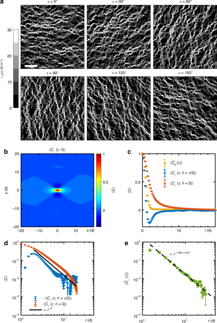
Fig. 3. Spatial distributions of polarized stress fields and their autocorrelation functions.

a Spatial distributions of six polarized stress fields τ₁(α). Scale bar = 10d. b Spatial autocorrelation map $⟨C_{{\tau }_1}\left(r,\theta \right)⟩$ of coarse-grained polarized stress τ₁(α), 〈 ⋯ 〉 denotes ensemble average over 100 configurations and different polarized angles α. Here, 〈C〉 denotes correlation functions. c Cuts of $⟨C_{{\tau }_1}\left(r,\theta \right)⟩$ along θ = 0, π/2 and autocorrelation function of coarse-grained pressure $⟨{\overline{C}}_p\left(r\right)⟩$, the over bar denotes average over θ. d Log-log plots of $⟨C_{{\tau }_1}\left(r,\theta =0\right)⟩$ and $-⟨C_{{\tau }_1}\left(r,\theta =\pi /2\right)⟩$. The solid line  ∝ r⁻² is guide to the eye. e The azimuthal averaged autocorrelation function of τ₁, $⟨{\overline{C}}_{{\tau }_1}\left(r\right)⟩$. The error bars represent the standard errors. The black dashed line indicates a power law fit of $⟨{\overline{C}}_{{\tau }_1}\left(r\right)⟩$ for r > 3d.