GENERALIZABLE MULTI-SITE TRAINING AND TESTING OF DEEP NEURAL NETWORKS USING IMAGE NORMALIZATION

Abstract

The ability of medical image analysis deep learning algorithms to generalize across multiple sites is critical for clinical adoption of these methods. Medical imging data, especially MRI, can have highly variable intensity characteristics across different individuals, scanners, and sites. However, it is not practical to train algorithms with data from all imaging equipment sources at all possible sites. Intensity normalization methods offer a potential solution for working with multi-site data. We evaluate five different image normalization methods on training a deep neural network to segment the prostate gland in MRI. Using 600 MRI prostate gland segmentations from two different sites, our results show that both intra-site and inter-site evaluation is critical for assessing the robustness of trained models and that training with single-site data produces models that fail to fully generalize across testing data from sites not included in the training.

1. INTRODUCTION

While deep learning methods are increasingly applied to medical image analysis tasks [1], challenges remain with respect to their clinical use. In clinical setups, robustness and generalizability are critical, especially given the differences in imaging equipment across sites. Typically in research, however, the data used to train and test these algorithms does not span the full range of clinical environments. It is not feasible to collect data across all clinical sites and all imaging equipment. This results in training and testing datasets that have limited numbers of samples, have homogeneous distributions of subjects, and have uniform data sources, e.g. using the same magnetic resonance (MR) imaging (MRI) scanner for all data. Overall, using data in this manner results in deep learning models that are tuned to specific training data.

While training with fully representative data from all hospitals may never be practical, an alternative strategy is to train specific models for very specific data acquisition protocols, e.g. one model per MR scanner at every clinical site for each clinical task. In this scenario, learned models may be shared across sites, but the model training is unique for individual clinical tasks. While transfer learning [2] and learning without forgetting [3] facilitate model training and model reuse, re-training models for every new piece of equipment and for every task is not practical either. Image normalization methods offer another solution for working with multi-site data.

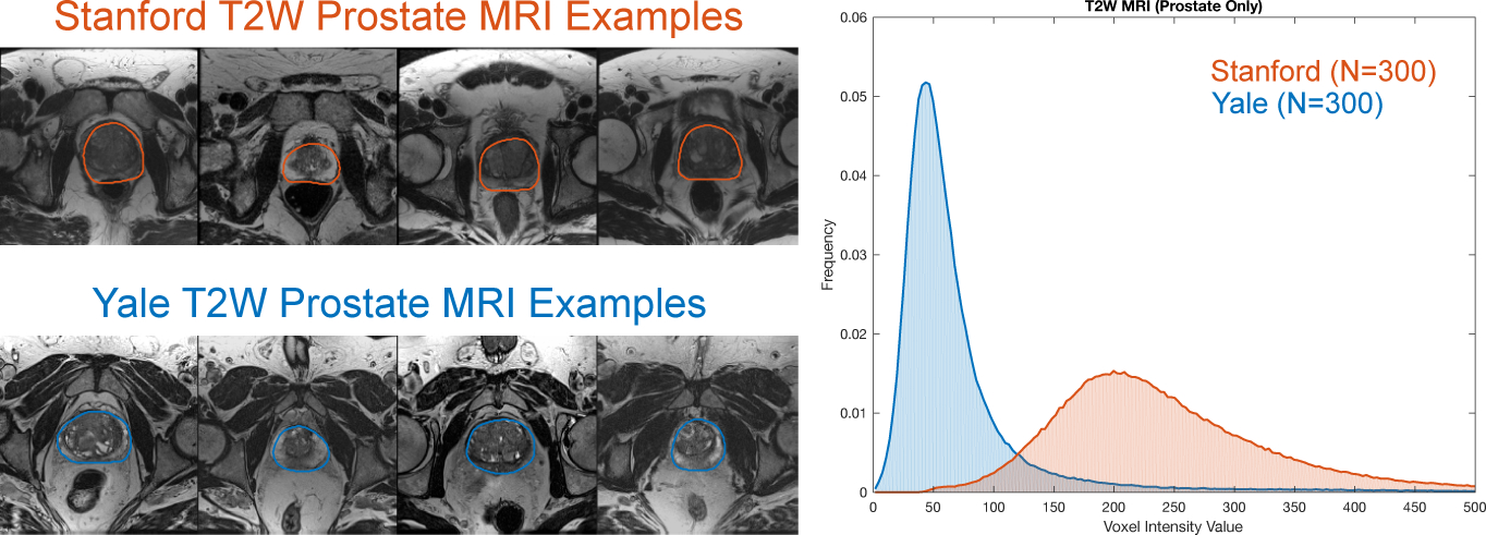
Data normalization is a key pre-processing step for machine learning algorithms. In natural images, changes in illumination and brightness contribute to intensity heterogeneity, however, the large number of image samples available to these applications makes training feasible and simply removing the dataset’s global mean intensity value from all pixels is empirically sufficient for deep neural networks with these types of images [4]. This is not possible with medical images that come from different equipment and can have vastly (or subtly) different image intensity characteristics. While deep learning has found success with CT imaging [5], which benefits from a standardized intensity scale across devices, MRI presents a challenge (even for simple tasks [6]). Not only do MR images from different patients exhibit variability in intensity distribution, but they exhibit variability across scanners and sites, e.g. different means and variances (Fig. 1). Medical imaging data is heterogeneous in terms of subject anatomy and limited in the number of samples. Therefore, per image normalization is necessary for medical images to account for differences in imaging hardware.

Fig. 1.

Example axial slices from T2W MR image volumes with manually segmented prostate glands from two sites: (top left) Stanford and (bottom left) Yale. (Right) The histograms of image intensity within the prostate gland (defined by the manual segmentations) for N = 300 subjects from each site show two distinct intensity profiles that result from using different MR scanners.

In this paper, we investigate the generalization of a deep learning prostate gland segmentation algorithm across multiple sites and we demonstrate the impact different normalization methods have on both intra-site and inter-site evaluation. Prostate segmentation in MRI is a well studied problem [7] subject to inter-site variability [8]. Here, we focus on training and testing a popular deep learning segmentation architecture using images from 600 subjects from two sites: Stanford and Yale. We show that (i) intra-site evaluation alone does not demonstrate algorithm generalizability, i.e. the algorithm can learn the intensity characteristics of a particular site but fail during prediction using data from a different site, (ii) image normalization has little effect on intra-site training but can be used to more robustly apply single-site models to multi-site data, and (iii) single-site training fails to learn models that generalize well across multi-site testing data, but image normalization can help.

2. METHODS

2.1. Image Normalization

Prior to the segmentation algorithm’s training and testing, we apply a normalization function f to each image to produce an intensity-normalized version of that image I’ = f(I). We test five different methods to perform image normalization: (i) None, which uses the raw intensity values and performs no normalization; (ii) Scaled, which scales the image intensities to have intensity values within the range [0, 1]; (iii) Gaussian, which shifts and scales the image intensity to have zero mean and unit variance; (iv) Quantile quantile normalization, which shifts the intensities to have zero median and unit interquartile range; and (v) Histogram matching, which is a non-linear mapping of image intensities to match a target distribution [9]. In this case, we create an idealized target distribution by averaging the median-centered histograms of all images from a single site (Yale). We then match the histograms from all other images (from both sites) to this target distribution. The Scaled, Gaussian, and Quantile normalization methods are linear transformations of the image intensity values, such that f(I) = αI + β, while the Histogram matching method performs a non-linear mapping. Fig. 1 shows the original MRI prostate intensity distributions without normalization and Fig. 2 shows the normalization results.

Fig. 2.

Histograms of T2W MRI intensity within the prostate gland (defined by manual segmentations) from two different sites: Stanford (orange) and Yale (blue) (N = 300 for each site). The distribution overlap has a profound effect on segmentation performance when training a deep neural network. Here, we show four different image normalization methods and their effect on the prostate gland intensity distribution: (from left to right) (i) adjusting the intensities to range between [0, 1] (Scaled); (ii) adjusting the intensities to have zero mean and unit variance (Gaussian); (iii) adjusting the intensities to have zero median and unit inter quartile range (Quantile); and (iv) performing histogram matching to a target distribution (Histogram). Fig. 1 shows the original intensity distributions prior to normalization.

2.2. Model Training and Segmentation

Given a set of N training images I = {I_i, M_i|i = 1, … , N}, where I_i denotes an anatomical MR image with a paired binary segmentation mask M_i, we train a deep neural network to perform prostate gland segmentation. We use a modified version of the U-Net [10] fully-convolutional network (FCN) architecture. Our implementation of this network differs from the standard U-Net architecture in that we used three max-pooling operations instead of the standard four, which results in a total of 18 convolutional layers (7,696,256 trainable parameters). We use a patch-based training approach, training with patch sizes of 128 × 128 pixels. For each training epoch, we randomly extracted 6,400 overlapping patches from the N images in the training data set. To augment our training set, we randomly flip patches left and right to take advantage of anatomical symmetries. We train with a mini-batch size of 64 patches and optimize the cross-entropy loss function using the Adam optimizer with initial learning rate 0.0005 with exponential decay 0.98. We used no dropout layers in the model in order to simplify the analysis of the data normalization. All models were trained for a total of 20,000 iterations.

To segment a test image I not included in the training set, we take advantage of the FCN architecture to adjust our patch size during inference to cover the entire image field. Here, we select a patch size of 256 × 256 to cover the entire image field of view for the largest images. This strategy to use larger patch sizes during inference helps avoid both the need for blending overlapping patches and the possibility of introducing edge artifacts at patch borders during prediction time. For images with dimensions less than 256, we mirror pad the images to fill the entire patch dimensions.

3. RESULTS AND DISCUSSION

From clinical databases at Stanford and Yale, we selected two sets of prostate MRI I_S and I_Y, respectively, each containing N = 300 subjects who underwent MR-guided prostate cancer biopsy. Stanford images were acquired on a 3T GE Discovery MR750 scanner and Yale images were acquired on a 3T Siemens Verio scanner. For each subject i = 1, … , N, we have an anatomical T2-weighted (T2W) MR image I_i acquired without an endorectal coil and a paired prostate gland segmentation M_i. This segmentation was performed by a radiologist as part of standard clinical practice using a semi-automated segmentation process [11] with the ProFuse imaging software (Eigen, Grass Valley, CA). The distribution (Mean±SD) of prostate volumes for Stanford and Yale was 59.3 ± 36.3 and 58.5 ± 35.8 cc, respectively. All data were anonymized. From the 3D image volumes, we extracted the central axial 2D slice of the prostate and the corresponding mask by computing the gland’s center of gravity (COG) from the mask and then selecting the 2D slice closest to the COG’s z-value. We resampled these midgland slices to have 1.0 mm isotropic spacing using linear interpolation for the T2W MRIs and nearest neighbor interpolation for the masks. Using this data, we tested the effect of different normalization methods (Sec. 2.1) on the segmentation performance of a deep neural network (Sec. 2.2) trained using data from a single site and from both sites. We evaluated segmentation performance by calculating the Dice overlap between the predicted prostate gland segmentation and the ground-truth segmentation mask. For each train-test pair, we assessed significance between pairwise comparisons of the normalization methods using a Wilcoxon signed rank test with a significance level of 0.05.

3.1. Single-site Training

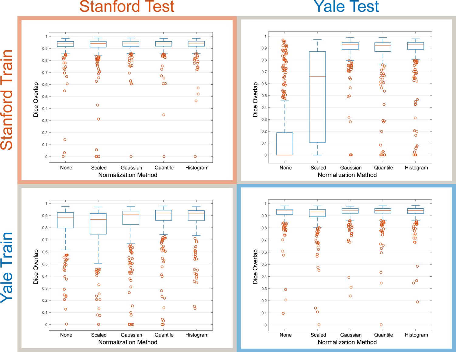
First, we evaluated both intra-site and inter-site segmentation performance of segmentation models trained using data from only a single site. For each site, we performed a 3-fold cross-validation study using N=200 subjects for training in each fold and using the remaining 100 images for testing such that all images in the set were tested once. Model training was repeated for each of the five different normalization methods. We performed intra-site testing by using the trained model from each fold to segment the 100 left-out test images from the same site. Additionally, we performed inter-site testing by using the trained model from each fold to segment 100 images from the other site. We repeated the same training and testing procedure for models and data from both sites.

Boxplots of the Dice overlap results (Fig. 3) illustrate the effect of each image normalization method for intraand inter-site segmentation performance. The choice of normalization method has a limited effect on the segmentation performance when testing on data from the same site. For intra-site testing, we observed statistically significant differences between Scaled and all other methods as well as None and Quantile normalization at Yale, and both None and Scaling normalization methods performed significantly worse than all other methods at Stanford. However, when testing on the data from a different site, the choice of image normalization method has a profound impact. This is illustrated most clearly in the case of testing Yale data on models trained with Stanford data, where using no normalization resulted in median Dice segmentation values of zero and Scaling resulted in highly variable segmentations significantly worse than other methods. For the best performing normalization methods in inter-site testing, we observed no significant differences between Gaussian and Histogram normalization for Stanford train-Yale test data, and no significant differences between Quantile and Histogram normalization for Yale train-Stanford test data. Overall, segmentation performance was worse for inter-site testing (Table 1), which indicated that models over-trained to the single-site data.

Fig. 3.

Intra-site and inter-site testing illustrates the importance of image normalization methods on prostate gland segmentation performance (Dice overlap) when training with data from a single site. We show results for models trained using Stanford images alone and tested on data from either Stanford or Yale, as well as results for models trained using Yale images alone and tested on data from either Stanford or Yale. Boxplots show the median, 25th and 75th percentiles, extremes (approximately the middle 99.3%), and outliers.

Table 1.

Intra-site, inter-site, and multi-site prostate segmentation results (Dice overlap (%)) using the Quantile normalization method on data from Stanford (S) and Yale (Y). Values are reported as Median (interquartile range).

Training Data	Testing Data
	S	Y	S+Y
S	0.944 (0.039)	0.924 (0.075)	0.935 (0.053)
Y	0.921 (0.085)	0.945 (0.040)	0.933 (0.056)
S+Y	0.944 (0.038)	0.944 (0.044)	0.944 (0.040)

3.2. Multi-site Training

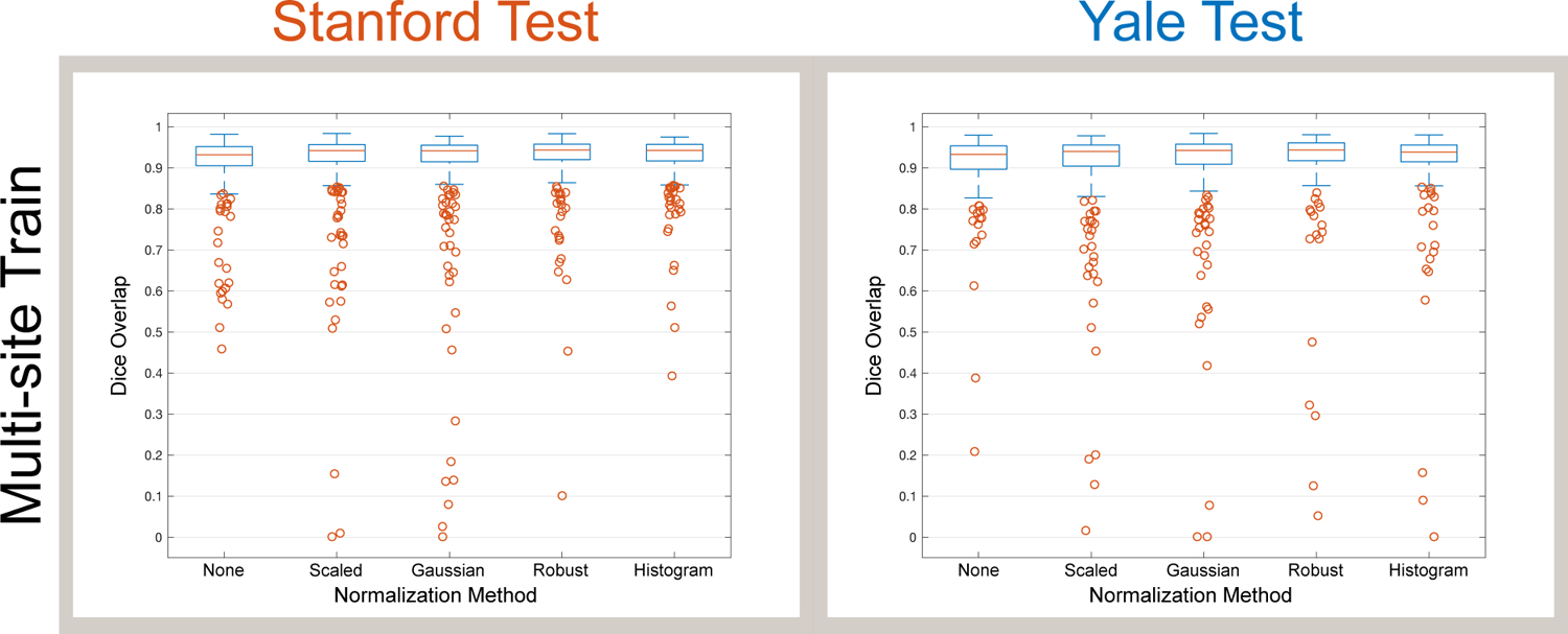
To evaluate the effect of including data from multiple sites in model training, we performed another set of 3-fold cross validation experiments. For each fold of multi-site training, we selected 100 subjects from Stanford and 100 subjects from Yale to form a training set I_S+Y with N = 200 subjects to train our model. For each testing fold in this setup, we selected 100 images from Stanford and 100 images from Yale to form a test set of 200 images such that each subject was tested only once among the 3 folds. Compared to the single-site training results, multi-site training results in much-improved performance when testing with data from multiple sites (Fig. 4). We observed that Quantile normalization produced the highest median Dice scores (0.944), which was significantly higher than all other normalization methods. Using Quantile normalization, Table 1 shows that multi-site training significantly improved multi-site testing results compared to single-site training.

Fig. 4.

Multi-site training results in much better segmentation performance (Dice overlap) across different sites compared to intra-site training (Fig. 3). Boxplots show the median, 25th and 75th percentiles, extremes (approximately the middle 99.3%), and outliers.

4. CONCLUSION

In this paper, we present an analysis of how well a particular deep neural network generalizes across different sites using different image normalization methods, which is a critical question to answer for algorithms in clinical use. We demonstrate segmentation results using 2D prostate MRI and we show that a Quantile normalization strategy appears to work well for this data. Here, the Quantile method centered the intensity distribution of the anatomy of interest (the prostate) to zero (Fig. 2) because it is robust to outlier intensities present in the rest of the image volume and it does not rely on the assumption of the intensities being Gaussian. In the future, we plan to apply this approach to other image segmentation tasks using different image modalities as well as to 3D data. In the future, we would like to test using more than two sites to investigate how many sites is enough to achieve general-izable model training. We also plan to incorporate the image normalization process directly into the model training procedure itself. We finally note, that a medical image is a function of both the scanner and the anatomy. Results obtained when training on a single scanner and evaluated on images from the same scanner can be artificially “inflated”, as these high dimensional deep neural networks have the flexibility to learn not only appearance but also the specific interactions of a given scanner and a structure. Conversely, as we demonstrate in this paper, such methods can yield unacceptable results when applied to images from a different scanner.