Semiparametric Bayesian variable selection for gene-environment interactions

Abstract

Many complex diseases are known to be affected by the interactions between genetic variants and environmental exposures beyond the main genetic and environmental effects. Study of gene-environment (G×E) interactions is important for elucidating the disease etiology. Existing Bayesian methods for G×E interaction studies are challenged by the high-dimensional nature of the study and the complexity of environmental influences. Many studies have shown the advantages of penalization methods in detecting G×E interactions in “large p, small n” settings. However, Bayesian variable selection, which can provide fresh insight into G×E study, has not been widely examined. We propose a novel and powerful semiparametric Bayesian variable selection model that can investigate linear and nonlinear G×E interactions simultaneously. Furthermore, the proposed method can conduct structural identification by distinguishing nonlinear interactions from main-effects-only case within the Bayesian framework. Spike-and-slab priors are incorporated on both individual and group levels to identify the sparse main and interaction effects. The proposed method conducts Bayesian variable selection more efficiently than existing methods. Simulation shows that the proposed model outperforms competing alternatives in terms of both identification and prediction. The proposed Bayesian method leads to the identification of main and interaction effects with important implications in a high-throughput profiling study with high-dimensional SNP data.

1 |. INTRODUCTION

It has been widely recognized that the genetic and environmental main effects alone are not sufficient to decipher an overall picture of the genetic basis of complex diseases. The gene-environment (G×E) interactions also play vital roles in dissecting and understanding complex diseases beyond the main effects.^1,2 Significant amount of efforts have been made to conducting analysis for the investigation of the associations between disease phenotypes and interaction effects marginally, especially in GWAS.³ As the disease etiology and prognosis are generally attributable to the coordinated effects of multiple genetic and environment factors, as well as the G×E interactions, joint analysis has provided a powerful alternative to dissect G×E interactions.

From the statistical modeling perspective, the interactions can be described as the product of variables corresponding to genetic and environmental factors. With the main G and E effects, as well as their interactions, the contribution of genetic variants to disease phenotype can be expressed as a linear function of the environmental factor. Such a linear interaction assumption does not necessarily hold true in practice. Taking the Nurses’ Health Study (NHS) data analyzed in this article as an example, we are interested in examining how the SNP effects on weight are mediated by age as the environmental factor. The range of subjects’ age in the NHS data is from 41 to 68. As reported, for type 2 diabetes (T2D), the average age for the onset is 45 years.⁴ Therefore, the presence of rs1106380×age interaction is roughly within such a range. We fit a Bayesian marginal model to SNP rs1106380 by using a nonparametric method to model the G×E interaction while accounting for effects from clinical covariates. A 95% credible region has also been provided. Figure 1 clearly suggests that the linear interaction assumption is violated. Misspecifying the form of interactions will lead to biased identification of important effects and inferior prediction performance.

FIGURE 1.

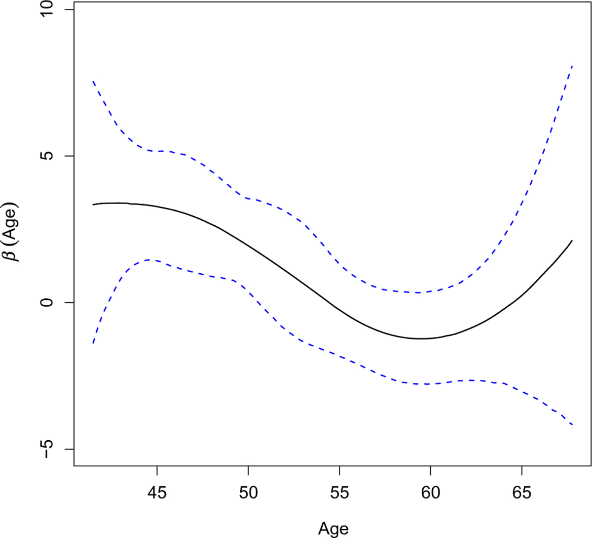
Nonlinear G×E effect of SNP rs1106380 from the Nurses’ Health Study (NHS) data. The blue dashed lines represent the 95% credible region

The nonlinear G×E interactions have been first conducted in marginal analysis, including those by Ma et al⁵ and Wu and Cui.⁶ Motivated by the set-based association analysis, the modeling strategy has been adopted to investigate how genetic variants in a set, such as the gene set, pathways, or networks, are mediated by one or multiple types of environmental exposures to influence disease risk. The set-based modeling incorporating the nonlinear G×E interactions is essentially a joint analysis with high-dimensional covariates. Recently, penalized variable selection methods have emerged as a promising tool to capture G×E interactions that might be only weak or moderate individually, but that are strong collectively.^7–12

Penalization methods have been first coined in the work of Tibshirani,¹³ which has also pointed out the connection between penalization and the corresponding Bayesian variable selection methods. In particular, the LASSO estimate can be interpreted as the posterior mode estimate when identical and independent Laplace prior has been imposed on each component of the coefficient vector under penalized least square loss. Park and Casella¹⁴ have further refined the prior as a conditional Laplace prior within the fully Bayesian framework to guarantee the unimodality of the posterior distribution. As LASSO belongs to the family of penalized estimate induced by the ${\mathcal{l}}_q$ norm penalty with q = 1, the Bayesian counterpart of penalization methods has been generalized to accommodate more complex data structure with other penalty functions, such as elastic net, fused LASSO, and group LASSO. These extensions can also be formulated within the Bayesian framework with a similar rationale of specifying priors.¹⁵

As penalization is tightly connected to Bayesian methods, the development of novel Bayesian variable selection will significantly broaden the scope of variable selection methods for G×E interaction studies, which will provide us fresh perspectives and promising results not offered by the existing studies. However, our limited literature review indicates that Bayesian variable selection has not been thoroughly conducted in existing G×E studies, especially for nonlinear interactions. For example, Liu et al¹⁶ have developed a Bayesian mixture model to identify important G×E and G×G interaction effects through indicator model selection. Variable selection has been achieved by examining the posterior inclusion probability. Under a two-phase sampling design, Ahn et al¹⁷ have considered Bayesian variable selection on G×E interactions using spike-and-slab priors. Both studies cannot handle nonlinear interactions. More pertinent to the penalization, Li et al¹⁸ have developed a Bayesian group LASSO for nonparametric varying coefficient models, where the nonlinear interaction is expressed as a linear combinations of Legendre polynomials, and the identification of G×E interactions amounts to the shrinkage selection of polynomials on the group level using multivariate Laplace priors. Li et al¹⁸ have built upon the Laplace prior adopted in Bayesian LASSO; therefore, the coefficients cannot be shrunken to zero exactly in order to achieve the “real” sparsity.

Accounting for nonlinear effects in G×E studies has deeply rooted in structured variable selection for high-dimensional data.¹⁹ An efficient selection procedure is expected to not only accurately pinpoint the form of nonlinear interactions but also avoid modeling the main-effect-only case (corresponding to the nonzero constant effects) as nonparametric ones, since this type of misspecification may overfit the data and result in loss of efficiency. To the best of our knowledge, automatic structure identification involving nonlinear effects has not been conducted in Bayesian G×E studies. To overcome the aforementioned limitations, we develop a novel semiparametric Bayesian variable selection method for G×E interactions. We consider both linear and nonlinear interactions simultaneously. The interactions between a genetic factor and a discrete environmental factor are modeled parametrically, while the nonlinear interactions are modeled using varying coefficient functions. In particular, we conduct automatic structure identification via Bayesian regularization to separate the cases of G×E interactions, main-effect-only and no genetic effects at all, which more flexibly captures the main and interaction effects. Besides, to shrink the coefficients of unimportant linear and nonlinear effects to zero exactly, we adopt the spike-and-slab priors in our model. The spike-and-slab priors have recently been shown as effective when being incorporated in Bayesian hierarchical framework for penalization methods, including the spike-and-slab LASSO,^20,21 Bayesian fused LASSO,²² and Bayesian sparse group LASSO.²³ It leads to sparsity in the sense of exact 0 posterior estimates which are not available in Bayesian LASSO type of Bayesian shrinkage methods including that in the work of Li et al.¹⁸

Motivated by the pressing need to conduct efficient Bayesian G×E interaction studies accounting for the nonlinear interaction effects, the proposed semiparametric model significantly advances from existing Bayesian variable selection methods for G×E interactions in the following aspects. First, compared to studies that solely focus on linear^16,17 or nonlinear effects,¹⁸ the proposed one can accommodate both types of effects concurrently; thus, more comprehensively describe the overall genetic architecture of complex diseases. Second, to the best of our knowledge, for G×E interactions, automatic structure discovery has been considered in the Bayesian framework for the first time. Compared to Li et al,¹⁸ one of the very few (or perhaps the only) literature in Bayesian variable selection for nonlinear effects, our method is more fine tuned for the structured sparsity by distinguishing whether the genetic variants have nonlinear interaction, main effects only, and no genetic effects at all, with the forms of coefficient functions being varying, nonzero constant, and zero, respectively. Third, borrowing strength from the spike-and-slab priors, we efficiently perform Bayesian shrinkage on the individual and group level simultaneously. In particular, with B-spline basis expansion, the identification of nonlinear interaction is equivalent to the selection of a group of basis functions. We develop an efficient MCMC algorithm for semiparametric Bayesian hierarchical model. We show in both simulations and a case study that the exact sparsity significantly improves accuracy in identification of relevant main and interaction effects, as well as prediction. For fast computation and reproducible research, we implement the proposed and alternative methods in C++ and encapsulate them in a publicly available R package spinBayes.²⁴

The rest of the article is organized as follows. In Section 2, we formulate the semiparametric Bayesian variable selection model and derive a Gibbs sampler to compute the posterior estimates of the coefficients. We carry out the simulation studies to demonstrate the utility of our method in Section 3. A case study of Nurses’ Health Study (NHS) data is conducted in Section 4.

2 |. DATA AND MODEL SETTINGS

2.1 |. Partially linear varying coefficient model

We denote the ith subject using subscript i. Let (X_i, Y_i, Z_i, E_i, W_i), i = 1, … , n, be independent and identically distributed random vectors. Y_i is the response variable. X_i is the p-dimensional design vector of genetic factors, and Z_i and E_i are the continuous and discrete environment factors, respectively. The clinical covariates are denoted by q-dimensional vector W_i. In the NHS data, the response variable is weight, and X_i represents SNPs. We consider age and the indicator of history of hypertension for Z_i and E_i, correspondingly. Height and total physical activity are used as clinical covariates, so q is 2. Now, consider the following partially linear varying coefficient model:

$$Y_i={\beta }_0\left(Z_i\right)+\sum _{j=1}^p{\beta }_j\left(Z_i\right)X_{ij}+\sum _{t=1}^q{\alpha }_t{W}_{it}+{\zeta }_0{E}_i+\sum _{j=1}^p{\zeta }_j{E}_i{X}_{ij}+{ϵ}_i,$$ (1)

where β_j(·) is a smoothing varying coefficient function, α_t is the coefficient of the tth clinical covariates, ζ₀ is the coefficient of the discrete E factor, and ζ_j is the coefficient of the interaction between the jth G factor X_j = (X_1j, … , X_nj)^⊤ and E_i. The random error ϵ_i ~ N(0, σ²).

Here, only two environmental factors, Z_i and E_i, are considered for the simplicity of notation. Their interactions with the G factor are modeled as nonlinear and linear forms, respectively. The model can be readily extended to accommodate multiple E factors.

2.2 |. Basis expansion for structure identification

As we discussed, distinguishing the case of main-effect-only from nonlinear G×E interaction is necessary since misspecification of the effects cause overfitting. The following basis expansion is necessary for the separation of different types of effects. We approximate the varying coefficient function β_j(Z_i) via basis expansion. Let q_n be the number of basis functions

$${\beta }_j\left(Z_i\right)\approx \sum _{k=1}^{q_n}{\tilde{B}}_{jk}\left(Z_i\right){\tilde{\gamma }}_{jk}={\tilde{B}}_j{\left(Z_i\right)}^{\top }{\tilde{\gamma }}_j,$$

where ${\tilde{B}}_j\left(Z_i\right)={\left({\tilde{B}}_{j1}\left(Z_i\right),\dots ,{\tilde{B}}_{j{q}_n}\left(Z_i\right)\right)}^{\top }$ is a set of normalized B-spline basis, and ${\tilde{\gamma }}_j={\left({\tilde{\gamma }}_{j1},\dots ,{\tilde{\gamma }}_{j{q}_n}\right)}^{\top }$ is the coefficient vector. By changing of basis, the aforementioned basis expansion is equivalent to

$${\beta }_j(\cdot )\approx \sum _{k=1}^{q_n}{\tilde{B}}_{jk}(\cdot ){\tilde{\gamma }}_{jk}\doteq {\gamma }_{j1}+{\tilde{B}}_{j*}{(\cdot )}^{\top }{\gamma }_{j*},$$

where ${\tilde{B}}_{j*}\left(Z_i\right)={\left({\tilde{B}}_{j2}\left(Z_i\right),\dots ,{\tilde{B}}_{j{q}_n}\left(Z_i\right)\right)}^{\top }\cdot {\gamma }_{j1}$ and ${\gamma }_{j*}={\left({\gamma }_{j2},\dots ,{\gamma }_{j{q}_n}\right)}^{\top }$ correspond to the constant and varying components of β_j(·), respectively. The intercept function can be approximated similarly as ${\beta }_0(\cdot )\approx {\sum }_{k=1}^{q_n}{\tilde{B}}_{0k}(\cdot ){\tilde{\eta }}_k\doteq {\eta }_1+{\tilde{B}}_{0*}{(\cdot )}^{\top }{\eta }_{*}$. Define γ_j = (γ_j1, (γ_j*)^⊤)^⊤, η = (η₁, (η_*)^⊤)^⊤, $B_j\left(Z_i\right)={\left(1,{\left({\tilde{B}}_{j*}\left(Z_i\right)\right)}^{\top }\right)}^{\top }\doteq {\left(B_{j1}\left(Z_i\right),\dots ,B_{j{q}_n}\left(Z_i\right)\right)}^{\top }$, and $B_0\left(Z_i\right)={\left(1,{\left({\tilde{B}}_{0*}\left(Z_i\right)\right)}^{\top }\right)}^{\top }$. Collectively, model (1) can be rewritten as

$$\begin{gathered} Y_i=B_0{\left(Z_i\right)}^{\top }\eta +\sum _{j=1}^p{B}_j{\left(Z_i\right)}^{\top }{\gamma }_j{X}_{ij}+\sum _{t=1}^q{\alpha }_t{W}_{it}+{\zeta }_0{E}_i+\sum _{j=1}^p{\zeta }_j{E}_i{X}_{ij}+{ϵ}_i \\ =B_0{\left(Z_i\right)}^{\top }\eta +\sum _{j=1}^p\left(X_{ij}{\gamma }_{j1}+U_{ij}^{\top }{\gamma }_{j*}\right)+W_i^{\top }\alpha +E_i^{\top }{\zeta }_0+T_i^{\top }\zeta +{ϵ}_i, \end{gathered}$$

where $U_{ij}={\left(B_{j2}\left(Z_i\right)X_{ij},\dots ,B_{j{q}_n}\left(Z_i\right)X_{ij}\right)}^{\top },\alpha ={\left({\alpha }_1,\dots ,{\alpha }_q\right)}^{\top },T_i={\left(X_{i1}{E}_i,\dots ,X_{ip}{E}_i\right)}^{\top }$, and ζ = (ζ₁, … , ζ_p)^⊤. Note that basis functions have been widely adopted for modeling the functional type of coefficient in general semiparametric models, as well as functional regression analysis.^25–27 For a comprehensive review of literature in this area, please refer to the work of Morris.²⁸

2.3 |. Semiparametric Bayesian variable selection

The proposed semiparametric model is of “large p, small n” nature. First, not all the main and interaction effects are associated with the phenotype. Second, we need to further determine for the genetic variants, whether they have nonlinear interactions, or main effect merely, or no genetic contribution to the phenotype at all. Therefore, variable selection is demanded.

From the Bayesian perspective, variable selection falls into the following four categories: (1) indicator model selection, (2) stochastic search variable selection, (3) adaptive shrinkage, and (4) model space method.²⁹ Among them, adaptive shrinkage methods solicit priors based on penalized loss function, which leads to sparsity in the Bayesian shrinkage estimates. For example, within the Bayesian framework, LASSO and group LASSO estimates can be understood as the posterior mode estimates when univariate and multivariate independent and identical Laplace priors are placed on the individual and group level of regression coefficients, respectively.^14,18

The proposed one belongs to the family of adaptive shrinkage Bayesian variable selection. For convenience of notation, we first define the approximated least square loss function as follows:

$$\tilde{L}\left(\eta ,\gamma ,\alpha ,{\zeta }_0,\zeta \right)={‖Y-B_0\eta -\sum _{j=1}^p{X}_j{\gamma }_{j1}-\sum _{j=1}^p{U}_j{\gamma }_{j*}-W\alpha -E{\zeta }_0-T\zeta ‖}^2,$$

where Y = (Y₁, … , Y_n)^⊤, B₀ = (B₀(Z₁), … , B₀(Z_n))^⊤, U_j = (U_1j, … , U_nj)^⊤, W = (W₁, … , W_n)^⊤, and T = (T₁, … , T_n)^⊤. Let θ = (η^⊤, γ^⊤, α^⊤, ζ₀, ζ^⊤)^⊤ be the vector of all the parameters. Then, the corresponding penalized loss function is

$$\tilde{L}\left(\eta ,\gamma ,\alpha ,{\zeta }_0,\zeta \right)+{\lambda }_e\sum _{j=1}^p\left|{\zeta }_j\right|+{\lambda }_c\sum _{j=1}^p\left|{\gamma }_{j1}\right|+{\lambda }_{\nu }\sum _{j=1}^p{‖{\gamma }_{j*}‖}_2.$$ (2)

The formulation of (2) has been primarily driven by the need to accommodate linear and nonlinear G×E interaction while avoiding misspecification of the main-effect-only as nonlinear interactions. Here, γ_j1 is the coefficient for the main effect of the jth genetic factor X_j, and the ${\mathcal{l}}_2$ norm of the spline coefficients ‖γ_j*‖₂ is corresponding to the varying parts of β_j(·). If ‖γ_j*‖₂ = 0, then there is no nonlinear interaction between X_j and continuous environment factor Z. Furthermore, if γ_j1 = 0, then X_j has no main effect and is not associated with the phenotype. Similarly, the linear interaction between X_j and the discrete environment factor E is determined by ζj. ζ_j = 0 indicates that there is no linear interaction. Overall, the penalty functions in (2) provide us the flexibility to achieve identification of structured sparsity through variable selection. Note that the main effects of environmental exposures Z and E are of low dimensionality; thus, they are not subject to selection. Therefore, for the current G×E interaction study, we are particular interested in conducting Bayesian variable selection on both the individual level of γ_j1 and ζ_j ( j = 1, … , p), and the group level of γ_j* ( j = 1, … , p).

Laplacian shrinkage on individual level effects.

Following the fully Bayesian analysis for LASSO proposed by Park and Casella,¹⁴ we impose the individual-level shrinkage on genetic main effects and linear G×E interactions by adopting i.i.d. conditional Laplace prior on γ_j1 and ζ_j (j = 1, … , p)

$$\begin{gathered} \pi \left({\gamma }_{11},\dots ,{\gamma }_{p1}\mid {\sigma }^2\right)=\prod _{j=1}^p\frac{{\lambda }_c}{2\sigma }\text{exp}\left\{-\frac{{\lambda }_c}{\sigma }\left|{\gamma }_{j1}\right|\right\} \\ \pi \left({\zeta }_1,\dots ,{\zeta }_p\mid {\sigma }^2\right)=\prod _{j=1}^p\frac{{\lambda }_e}{2\sigma }\text{exp}\left\{-\frac{{\lambda }_e}{\sigma }\left|{\zeta }_j\right|\right\}. \end{gathered}$$ (3)

The above Laplace priors can be expressed as scale mixture of normals³⁰

$$\begin{gathered} \pi {\left({\gamma }_{j1}\mid {\tau }_{cj}^2,{\sigma }^2\right)}^{\underset{~}{inv}}\text{N}\left(0,{\sigma }^2{\tau }_{cj}^2\right){\tau }_{cj}^2{}^{\underset{~}{inv}}\frac{{\lambda }_c^2}{2}\text{exp}\left\{-\frac{{\lambda }_c^2}{2}{\tau }_{cj}^2\right\} \\ \pi {\left({\zeta }_j\mid {\tau }_{ej}^2,{\sigma }^2\right)}^{\underset{~}{inv}}\text{N}\left(0,{\sigma }^2{\tau }_{ej}^2\right){\tau }_{ej}^2{}^{\underset{~}{inv}}\frac{{\lambda }_e^2}{2}\text{exp}\left\{-\frac{{\lambda }_e^2}{2}{\tau }_{ej}^2\right\}. \end{gathered}$$ (4)

It is easy to show that, after integrating out ${\tau }_{\mathit{\text{cj}}}^2$ and ${\tau }_{\mathit{\text{ej}}}^2$, (4) leads to the same priors in (3).

Laplacian shrinkage on group level effects.

Kyung et al¹⁵ extended the Bayesian LASSO to a more general form that can represent the group LASSO by adopting a multivariate Laplace prior. We follow the strategy and let the prior for γ_j* (j = 1, … , p) be

$$\pi \left({\gamma }_{j*}\mid {\sigma }^2\right)\propto \text{exp}\left\{-\frac{\sqrt{L}{\lambda }_v}{\sigma }{‖{\gamma }_{j*}‖}_2\right\},$$ (5)

where L = q_n – 1 is the size of the group, ${\left(\frac{\sqrt{L}{\lambda }_v}{\sigma }\right)}^{-1}$ is the scale parameter of the multivariate Laplace, and $\sqrt{L}$ terms adjust the penalty for the group size. $\sqrt{L}$ can be dropped from the formula when all the groups have the same size. In this study, we use the same number of basis functions for all parameters, and thus, L is the same for all groups. For completeness, we still include completeness, we still include in (5) for possible extension to varying group sizes in the future. Similar to the (4), this prior can be expressed as a gamma mixture of normal

$$\pi {\left({\gamma }_{j*}\mid {\tau }_{vj}^2,{\sigma }^2\right)}^{\underset{~}{inv}}{\text{N}}_L\left(0,{\sigma }^2{\tau }_{vj}^2{I}_L\right){\tau }_{vj}^2{}^{\underset{~}{inv}}\text{Gamma}\left(\frac{L+1}{2},\frac{L{\lambda }_v^2}{2}\right).$$ (6)

where $\frac{L+1}{2}$ is the shape parameter and $\frac{L{\lambda }^2}{2}$ is the rate parameter of the Gamma distribution. After integrating out ${\tau }_{vj}^2$ in (6), the conditional prior on γ_j* has the desired form in (5). Priors in (4) and (6) can lead to a similar performance as the general LASSO model in (2), by imposing individual shrinkage on γ_j1 and ζ_j and group level shrinkage on γ_j*, respectively.

Spike-and-slab priors on both individual and group level effects.

Compared with (2), priors in (4) and (6) cannot shrink the posterior estimates to exact 0. Li et al¹⁸ have such a limitation since multivariate Laplace priors have been imposed on the group level effects. One of the significant advancements of our study over existing Bayesian G×E interaction studies, including the work of Li et al,¹⁸ is the incorporation of spike-and-slab priors to achieve sparsity. For γ_j*, we have

$${\gamma }_{j*}\mid {\varphi }_{vj},{\tau }_{vj}^2,{\sigma }^2{}^{\underset{~}{inv}}{\varphi }_{vj}{\text{N}}_L\left(0,\text{diag}\left({\sigma }^2{\tau }_{vj}^2,\dots ,{\sigma }^2{\tau }_{vj}^2\right)\right)+\left(1-{\varphi }_{vj}\right){\delta }_0\left({\gamma }_{j*}\right){\varphi }_{vj}\mid {\pi }_v{}^{\underset{~}{inv}}\text{Bernoulli}\left({\pi }_v\right){\tau }_{vj}^2\mid {\lambda }_v{}^{\underset{~}{inv}}\text{Gamma}\left(\frac{L+1}{2},\frac{L{\lambda }_v^2}{2}\right),$$ (7)

where δ₀(γ_j*) denotes a point mass at 0_L×1 and π_v ∈ [0, 1]. We introduce a latent binary indicator variable ϕ_vj for each group j, (j = 1, … , p). ϕ_vj facilitates the variable selection by indicating whether or not the jth group is included in the final model. Specifically, when ϕ_vj = 0, the coefficient vector γ_j* has a point mass density at zero which implies all predictors in the jth group are excluded from the final model. This is equivalent to concluding that the jth G factor X_j does not have an interaction effect with the environment factor Z. On the other hand, when ϕ_vj = 1, the prior in (7) reduces to the prior in (6) and induces the same behavior as Bayesian group LASSO. Thus, the coefficients in vector γ_j* have nonzero values and the jth group is included in the final model. Note that, after integrating out ϕ_vj and ${\tau }_{vj}^2$ in (7), the marginal prior on γ_j* is a mixture of a multivariate Laplace and a point mass at 0_L×1 as follows:

$$\pi \left({\gamma }_{j*}\mid {\sigma }^2\right)~{\pi }_v\text{ M-Laplace }\left(0,\frac{\sigma }{\sqrt{L}{\lambda }_v}\right)+\left(1-{\pi }_v\right){\delta }_0\left({\gamma }_{j*}\right).$$ (8)

When π_v = 1, (8) is equivalent to (5). Fixing π_v = 0.5 makes the prior essentially noninformative since it gives the equal prior probabilities to all submodels. Instead of fixing π_v, we assign it a conjugate beta prior π_v ~ Beta(r_v, w_v) with fixed parameters r_v and w_v. The value of λ_v controls the shape of the slab part of (8) and determines the amount of shrinkage on the γ_j*. For computation convenience, we assign a conjugate Gamma hyperprior ${\lambda }_v^2~\text{Gamma}\left(a_v,b_v\right)$ that can automatically accounts for the uncertainty in choosing λ_v and ensure it is positive. We set a_v and b_v to small values so that the priors are essentially noninformative.

Remark. The form in (8) shows that our prior combines the strength of the Laplacian shrinkage and the spike-and-slab prior. The Laplacian shrinkage is used as the slab part of the prior, which captures the signal in the data and provides the estimation for large effects. Compared with (5), the additional spike part (point mass at zero) in (8) shrinks the negligibly small effects to zeros and achieve the variable selection.

Likewise, for γ_j1 and ζ_j (j = 1, … , p) corresponding to the individual level effects, the spike-and-slab priors can be written as

$${\gamma }_{j1}\mid {\varphi }_{cj},{\tau }_{cj}^2,{\sigma }^2{}^{\underset{~}{inv}}{\varphi }_{cj}\text{N}\left(0,{\sigma }^2{\tau }_{cj}^2\right)+\left(1-{\varphi }_{cj}\right){\delta }_0\left({\gamma }_{j1}\right){\varphi }_{cj}\mid {\pi }_c{}^{\underset{~}{inv}}\text{Bernoulli}\left({\pi }_c\right){\tau }_{cj}^2\mid {\lambda }_c{}^{\underset{~}{inv}}\text{Gamma}\left(1,\frac{{\lambda }_c^2}{2}\right)$$ (9)

$${\zeta }_j\mid {\varphi }_{ej},{\tau }_{ej}^2,{\sigma }^2{}^{\underset{~}{inv}}{\varphi }_{ej}\text{N}\left(0,{\sigma }^2{\tau }_{ej}^2\right)+\left(1-{\varphi }_{ej}\right){\delta }_0\left({\zeta }_j\right){\varphi }_{ej}\mid {\pi }_e{}^{{}^{\underset{~}{inv}}}\text{ Bernoulli }\left({\pi }_e\right){\tau }_{ej}^2\mid {\lambda }_e{}^{{}^{\underset{~}{inv}}}\text{Gamma}\left(1,\frac{{\lambda }_e^2}{2}\right).$$ (10)

We assign conjugate beta prior π_c ~ Beta(r_c, w_c) and π_e ~ Beta(r_e, w_e), and Gamma priors ${\lambda }_c^2~\text{Gamma}\left(a_c,b_c\right)$ and ${\lambda }_e^2~\text{Gamma}\left(a_e,b_e\right)$. An inverted gamma prior for σ² can maintain conjugacy. The limiting improper prior π(σ²) = 1∕σ² is another popular choice. Parameters η, α, and ζ₀ may be given independent flat priors.

2.4 |. Gibbs sampler

The binary indicator variables can cause an absorbing state in the MCMC algorithm that violates the convergence condition.³¹ To avoid this problem, we integrate out the indicator variables ϕ_c, ϕ_v, and ϕ_e in (7), (9), and (10). We will show that, even though ϕ_c, ϕ_v, and ϕ_e are not part of the MCMC chain, their values still can be easily computed at every iterations. Let μ = E(Y), the joint posterior distribution of all the unknown parameters conditional on data can be expressed as

$$\pi \left(\eta ,\alpha ,{\zeta }_0,{\gamma }_{j1},{\tau }_c^2,{\pi }_c,{\lambda }_c,{\gamma }_{j*},{\tau }_v^2,{\pi }_v,{\lambda }_v,{\zeta }_j,{\pi }_e,{\lambda }_e,{\tau }_e^2,{\sigma }^2\mid Y\right)\propto {\left({\sigma }^2\right)}^{-\frac{n}{2}}\text{exp}\left\{-\frac{1}{2{\sigma }^2}{(Y-\mu )}^{\top }(Y-\mu )\right\}\times \text{exp}\left(-\frac{1}{2}{\eta }^{\top }{\Sigma }_{\eta 0}^{-1}\eta \right)\text{exp}\left(-\frac{1}{2}{\alpha }^{\top }{\Sigma }_{\alpha 0}^{-1}\alpha \right)\text{exp}\left(-\frac{1}{2{\sigma }_{{\zeta }_0}^2}{\zeta }_0^2\right)\times \prod _{j=1}^p\left({\pi }_v{\left(2\pi {\sigma }^2{\tau }_{vj}^2\right)}^{-\frac{L}{2}}\text{exp}\left(-\frac{1}{2{\sigma }^2{\tau }_{vj}^2}{\gamma }_{j*}^{\top }{\gamma }_{j*}\right)I_{\left\{{\gamma }_{j*}\ne 0\right\}}+\left(1-{\pi }_v\right){\delta }_0\left({\gamma }_{j*}\right)\right)\times {\left({\lambda }_v^2\right)}^{a_v-1}\text{exp}\left(-b_v{\lambda }_v^2\right)\prod _{j=1}^p{\left(\frac{L{\lambda }_v^2}{2}\right)}^{\frac{L+1}{2}}{\left({\tau }_{vj}^2\right)}^{\frac{L+1}{2}-1}\text{exp}\left(-\frac{L{\lambda }_v^2}{2}{\tau }_{vj}^2\right)\times {\pi }_v^{{\gamma }_v-1}{\left(1-{\pi }_v\right)}^{w_v-1}\times \prod _{j=1}^p\left({\pi }_c{\left(2\pi {\sigma }^2{\tau }_{cj}^2\right)}^{-\frac{1}{2}}\text{exp}\left(-\frac{1}{2{\sigma }^2{\tau }_{cj}^2}{\gamma }_{j1}^2\right)I_{\left\{{\gamma }_{j1}\ne 0\right\}}+\left(1-{\pi }_c\right){\delta }_0\left({\gamma }_{j1}\right)\right)\times {\left({\lambda }_c^2\right)}^{a_c-1}\text{exp}\left(-b_c{\lambda }_c^2\right)\prod _{j=1}^p\frac{{\lambda }_c^2}{2}\text{exp}\left(-\frac{{\lambda }_c^2}{2}{\tau }_{cj}^2\right)\times {\pi }_c^{{\gamma }_c-1}{\left(1-{\pi }_c\right)}^{w_c-1}\times \prod _{j=1}^p\left({\pi }_e{\left(2\pi {\sigma }^2{\tau }_{ej}^2\right)}^{-\frac{1}{2}}\text{exp}\left(-\frac{1}{2{\sigma }^2{\tau }_{ej}^2}{\zeta }_j^2\right)I_{\left\{{\zeta }_j\ne 0\right\}}+\left(1-{\pi }_e\right){\delta }_0\left({\zeta }_j\right)\right)\times {\left({\lambda }_e^2\right)}^{a_e-1}\text{exp}\left(-b_e{\lambda }_e^2\right)\prod _{j=1}^p\frac{{\lambda }_e^2}{2}\text{exp}\left(-\frac{{\lambda }_e^2}{2}{\tau }_{ej}^2\right)\times {\pi }_e^{{\gamma }_e-1}{\left(1-{\pi }_e\right)}^{w_e-1}\times {\left({\sigma }^2\right)}^{-s-1}\text{exp}\left(-\frac{h}{{\sigma }^2}\right).$$

Let μ_(−η) = E(Y) − B₀η, representing the mean effect without the contribution of β₀(Z_i). The posterior distribution of η conditional on all other parameters can be expressed as

$$\pi (\eta \mid \text{ rest })\propto \pi (\eta )\pi (y\mid \cdot )\propto \text{exp}\left(-\frac{1}{2}{\eta }^{\top }{\Sigma }_{\eta 0}^{-1}\eta \right)\text{exp}\left(-\frac{1}{2{\sigma }^2}{(Y-\mu )}^{\top }(Y-\mu )\right)\propto \text{exp}\left(-\frac{1}{2}{\eta }^{\top }{\Sigma }_{\eta 0}^{-1}\eta -\frac{1}{2{\sigma }^2}{\left(Y-B_0\eta -{\mu }_{(-\eta )}\right)}^{\top }\left(Y-B_0\eta -{\mu }_{(-\eta )}\right)\right)\propto \text{exp}\left({\eta }^{\top }\left({\Sigma }_{\eta 0}^{-1}+\frac{1}{{\sigma }^2}{B}_0^{\top }{B}_0\right)\eta -\frac{2}{{\sigma }^2}{\left(Y-{\mu }_{(-\eta )}\right)}^{\top }{B}_0\eta \right).$$

Hence, the full conditional distribution of m is multivariate normal N(μ_η, Σ_η) with mean

$${\mu }_{\eta }={\left({\Sigma }_{\eta 0}^{-1}+\frac{1}{{\sigma }^2}{B}_0^{\top }{B}_0\right)}^{-1}{\left(\frac{1}{{\sigma }^2}{\left(Y-{\mu }_{(-\eta )}\right)}^{\top }{B}_0\right)}^{\top }$$

and variance

$${\Sigma }_{\eta }={\left({\Sigma }_{\eta 0}^{-1}+\frac{1}{{\sigma }^2}{B}_0^{\top }{B}_0\right)}^{-1}.$$

The full conditional distribution of α and ζ₀ can be obtained in similar way

$$\alpha \mid \text{ rest }~{\text{N}}_q\left({\mu }_{\alpha },{\Sigma }_{\alpha }\right),$$

where ${\mu }_{\alpha }={\Sigma }_{\alpha }{\left(\frac{1}{{\sigma }^2}{\left(Y-{\mu }_{(-\alpha )}\right)}^{\top }W\right)}^{\top }$ and ${\Sigma }_{\alpha }={\left({\Sigma }_{\alpha 0}^{-1}+\frac{1}{{\sigma }^2}{W}^{\top }W\right)}^{-1}$

$${\zeta }_0\mid \text{ rest }~N\left({\mu }_{{\zeta }_0},{\Sigma }_{{\zeta }_0}\right),$$

where ${\mu }_{{\zeta }_0}={\Sigma }_{{\zeta }_0}\left(\frac{1}{{\sigma }^2}{\left(Y-{\mu }_{\left(-{\zeta }_0\right)}\right)}^{\top }E\right)$ and ${\Sigma }_{{\zeta }_0}={\left(1/{\sigma }_{{\zeta }_0}^2+\frac{{\sum }_{i=1}^n{E}_i^2}{{\sigma }^2}\right)}^{-1}$.

Donote ${\mu }_{\left(-{\gamma }_{j*}\right)}=E(Y)-U_j{\gamma }_{j*}$ and l_vj = π(γ_j* ≠ 0|rest), the conditional posterior distribution of γ_j* is a multivariate spike-and-slab distribution

$${\gamma }_{j*}\mid \text{ rest }~l_{vj}\text{N}\left({\mu }_{{\gamma }_{j*},},{\sigma }^2{\Sigma }_{{\gamma }_{j*}}\right)+\left(1-l_{vj}\right){\delta }_0\left({\gamma }_{j*}\right),$$ (11)

where ${\mu }_{{\gamma }_{j*}}={\Sigma }_{{\gamma }_{j*}}{U}_j^{\top }\left(Y-{\mu }_{\left(-{\gamma }_{j*}\right)}\right)$ and ${\Sigma }_{{\gamma }_j*}={\left(U_j^{\top }{U}_j+\frac{1}{{\tau }_{vj}^2}{I}_L\right)}^{-1}$. It is easy to compute that l_vj is equal to

$$l_{vj}=\frac{{\pi }_v}{{\pi }_v+\left(1-{\pi }_v\right){\left({\tau }_{vj}^2\right)}^{\frac{L}{2}}{\left|{\Sigma }_{{\gamma }_{j*}}\right|}^{-\frac{1}{2}}\text{exp}\left(-\frac{1}{2{\sigma }^2}{‖{\sum }_{{\gamma }_{j*}}^{\frac{1}{2}}{U}_j^{\top }\left(Y-{\mu }_{\left(-{\gamma }_{j*}\right)}\right)‖}_2^2\right)}.$$

The posterior distribution (11) is a mixture of a multivariate normal and a point mass at 0. Specifically, at the gth iteration of MCMC, ${\gamma }_{j*}^{(g)}$ is drawn from $N\left({\mu }_{{\gamma }_{j*}},{\Sigma }_{{\gamma }_{j*}}\right)$ with probability l_vj and is set to 0 with probability 1 − l_vj. If ${\gamma }_{j*}^{(g)}$ is set to 0, we have ${\varphi }_{vj}^{(g)}=0$. Otherwise ${\varphi }_{vj}^{(g)}=1$.

Likewise, the conditional posterior distributions of γ_j1 and ζ_j are also spike-and-slab distributions. Let ${\mu }_{{\gamma }_{j1}}={\Sigma }_{{\gamma }_{j1}}{X}_j^{\top }\left(Y-{\mu }_{\left(-{\gamma }_{j1}\right)}\right)$ and ${\Sigma }_{{\gamma }_{j1}}={\left(X_j^{\top }{X}_j+\frac{1}{{\tau }_{cj}^2}\right)}^{-1}$, the full conditional distribution of γ_j1 is

$${\gamma }_{j1}\mid \text{ rest }~l_{cj}\text{N}\left({\mu }_{{\gamma }_{j1}},{\sigma }^2{\Sigma }_{{\gamma }_{j1}}\right)+\left(1-l_{cj}\right){\delta }_0\left({\gamma }_{j1}\right),$$

where

$$\begin{gathered} l_{cj}=\pi \left({\gamma }_{j1}\ne 0\mid \text{ rest }\right) \\ =\frac{{\pi }_c}{{\pi }_c+\left(1-{\pi }_c\right){\left({\tau }_{cj}^2\right)}^{\frac{1}{2}}{\left({\Sigma }_{{\gamma }_{j1}}\right)}^{-\frac{1}{2}}\text{exp}\left(-\frac{1}{2{\sigma }^2}{\Sigma }_{{\gamma }_{j1}}{‖{\left(Y-{\mu }_{\left(-{\gamma }_{j1}\right)}\right)}^{\top }{X}_j‖}_2^2\right)}. \end{gathered}$$

Let ${\mu }_{{\zeta }_j}={\Sigma }_{{\zeta }_j}{\left(Y-{\mu }_{\left(-{\zeta }_j\right)}\right)}^{\top }{T}_j$ and ${\Sigma }_{{\zeta }_j}={\left(T_j^{\top }{T}_j+\frac{1}{{\tau }_{ej}^2}\right)}^{-1}$, the full conditional distribution of ζ_j is

$${\zeta }_j\mid \text{ rest }~l_{ej}\text{N}\left({\mu }_{{\zeta }_j},{\sigma }^2{\Sigma }_{{\zeta }_j}\right)+\left(1-l_{ej}\right){\delta }_0\left({\zeta }_j\right),$$

where

$$\begin{gathered} l_{ej}=\pi \left({\zeta }_j\ne 0\mid \text{ rest }\right) \\ =\frac{{\pi }_e}{{\pi }_e+\left(1-{\pi }_e\right){\left({\tau }_{ej}^2\right)}^{\frac{1}{2}}{\left({\Sigma }_{{\zeta }_j}\right)}^{-\frac{1}{2}}\text{exp}\left(-\frac{1}{2{\sigma }^2}{\Sigma }_{{\zeta }_j}{‖{\left(Y-{\mu }_{\left(-{\zeta }_j\right)}\right)}^{\top }{T}_j‖}_2^2\right)}. \end{gathered}$$

At the gth iteration, the values of ${\varphi }_{cj}^{(g)}$ and ${\varphi }_{ej}^{(g)}$ can be determined by whether the ${\gamma }_{j1}^{(g)}$ and ${\zeta }_j^{(g)}$ are set to 0 or not, respectively. We list the conditional posterior distributions of other unknown parameters here. The details can be found in the Supplementary Materials.

$${\left({\tau }_{vj}^2\right)}^{-1}\mid \text{rest }~\left\{\begin{array}{ll}\text{ Inverse-Gamma }\left(\frac{L+1}{2},\frac{L{\lambda }_v^2}{2}\right),\hfill & \text{ if }{\gamma }_{j*}=0\hfill \\ \text{ Inverse-Gaussian }\left(L{\lambda }_v^2,\sqrt{\frac{L{\lambda }_v^2{\sigma }^2}{{‖{\gamma }_{j*}‖}_2^2}}\right),\hfill & \text{ if }{\gamma }_{j*}\ne 0\hfill \end{array}\right.$$

$${\left({\tau }_{cj}^2\right)}^{-1}\mid \text{rest }~\{\begin{array}{ll}\text{ Inverse-Gamma }\left(1,\frac{{\lambda }_c^2}{2}\right),\hfill & \text{ if }{\gamma }_{j1}=0\hfill \\ \text{ Inverse-Gaussian }\left({\lambda }_c^2,\sqrt{\frac{{\lambda }_c^2{\sigma }^2}{{\gamma }_{j1}^2}}\right),\hfill & \text{ if }{\gamma }_{j1}\ne 0\hfill \end{array}$$

$${\left({\tau }_{ej}^2\right)}^{-1}\mid \text{rest }~\{\begin{array}{ll}\text{ Inverse-Gamma }\left(1,\frac{{\lambda }_e^2}{2}\right),\hfill & \text{ if }{\zeta }_j=0\hfill \\ \text{ Inverse-Gaussian }\left({\lambda }_e^2,\sqrt{\frac{{\lambda }_e^2{\sigma }^2}{{\zeta }_j^2}}\right),\hfill & \text{ if }{\zeta }_j\ne 0\hfill \end{array}$$

${\lambda }_v^2$, ${\lambda }_c^2$, and ${\lambda }_e^2$ all have Gamma posterior distributions

$${\lambda }_v^2\mid \text{ rest }~\text{ Gamma }\left(a_v+\frac{p(L+1)}{2},b_v+\frac{L{\sum }_{j=1}^p{\tau }_{vj}^2}{2}\right)$$

$${\lambda }_c^2\mid \text{ rest }~\text{ Gamma }\left(a_c+p,b_c+\frac{{\sum }_{j=1}^p{\tau }_{cj}^2}{2}\right)$$

$${\lambda }_e^2\mid \text{ rest }~\text{ Gamma }\left(a_e+p,b_e+\frac{{\sum }_{j=1}^p{\tau }_{ej}^2}{2}\right).$$

π_v, π_c, and π_e have beta posterior distributions

$${\pi }_v\mid \text{ rest }~\text{Beta}\left(r_v+\sum _{j=1}^p{I}_{\left\{{\gamma }_j*=0\right\}},w_v+\sum _{j=1}^p{I}_{\left\{{\gamma }_{j*}\ne 0\right\}}\right)$$

$${\pi }_c\mid \text{ rest }~\text{Beta}\left(r_c+\sum _{j=1}^p{I}_{\left\{{\gamma }_{j1}=0\right\}},w_c+\sum _{j=1}^p{I}_{\left\{{\gamma }_{j1}\ne 0\right\}}\right)$$

$${\pi }_e\mid \text{ rest }~\text{Beta}\left(r_e+\sum _{j=1}^p{I}_{\left\{{\zeta }_j=0\right\}},w_e+\sum _{j=1}^p{I}_{\left\{{\zeta }_j\ne 0\right\}}\right).$$

Last, the full conditional distribution for σ² the posterior distribution for σ² is $\text{ Inverse-Gamma }\left({\mu }_{{\sigma }^2},{\Sigma }_{{\sigma }^2}\right)$ where

$${\sigma }^2\mid \text{ rest }~\text{ Inverse-Gamma }\left({\mu }_{{\sigma }^2},{\Sigma }_{{\sigma }^2}\right)$$

with mean

$${\mu }_{{\sigma }^2}=s+\frac{n+\sum I_{\left\{{\gamma }_{j1}\ne 0\right\}}+L\sum I_{\left\{{\gamma }_{j*}\ne 0\right\}}+\sum I_{\left\{{\zeta }_j\ne 0\right\}}}{2}$$

and variance

$${\Sigma }_{{\sigma }^2}=h+\frac{{(Y-\mu )}^{\top }(Y-\mu )+\sum _{j=1}^p\left({\left({\tau }_{cj}^2\right)}^{-1}{\gamma }_{j1}^2+{\left({\tau }_{vj}^2\right)}^{-1}{\gamma }_{j*}^{\top }{\gamma }_{j*}+{\left({\tau }_{ej}^2\right)}^{-1}{\zeta }_j^2\right)}{2}.$$

Under our priors’ setting, conditional posterior distributions of all unknown parameters have closed forms by conjugacy. Therefore, efficient Gibbs sampler can be used to simulate from the posterior distribution.

To facilitate fast computation and reproducible research, we have implemented the proposed and all the alternative methods in C++ from the R package spinBayes²⁴ available from the corresponding author’s GitHub website. The package is pending a manual inspection and will be available at CRAN soon.

3 |. SIMULATION

We compare the performance of the proposed method, Bayesian spike-and-slab variable selection with structural identification, termed as BSSVC-SI, to four alternatives termed as BSSVC, BVC-SI, BVC, and BL, respectively. BSSVC is the proposed method but without implementing structural identification. It does not distinguish the nonzero constant effect from the nonlinear effect. Specifically, in BSSVC, coefficients of q_n basis functions of β_j are treated as one group and are subject to selection at the group level. Comparison of BSSVC-SI with BSSVC demonstrate the importance of structural identification in the detection of interaction effects. BVC-SI is similar to the proposed method, except that it does not adopt the spike-and-slab prior. BVC does not use the spike-and-slab prior and does not distinguish the constant and varying effects. All these three alternative methods, BSSVC, BVC-SI, and BVC, are different variations of the proposed BSSVC-SI, aiming to evaluate the strength of using the spike-and-slab prior and demonstrate the necessity of including structural identification. The last alternative BL is the well-known Bayesian LASSO.¹⁴ BL assumes that all interactions are linear. Details of the alternatives, including the prior and posterior distributions, are available in the Supplementary Materials.

We consider four examples in our simulations. Under all four settings, the responses are generated from model (1) with n = 500, p = 100, and q = 2. Note that, the dimension of regression coefficients to be estimated after basis expansion is larger than the sample size (n = 500). For example, when the number of basis function q_n = 5, the effective dimension of regression coefficient is 604. In each example, we assess the performance in terms of identification, estimation, and prediction accuracy. We use the integrated mean squared error (IMSE) to evaluate estimation accuracy on the nonlinear effects. Let ${\widehat{\beta }}_j(z)$ be the estimate of a nonparametric function β_j(z), and ${\left\{z_m\right\}}_{m=1}^{n_{\mathit{\text{grid}}}}$ be the grid points where β_j is assessed. The IMSE of ${\widehat{\beta }}_j(z)$ is defined as $\text{IMSE}\left({\widehat{\beta }}_j(z)\right)=\frac{1}{n_{\mathit{\text{grid }}}}{\sum }_{m=1}^{n_{\mathit{\text{grid }}}}{\left\{{\widehat{\beta }}_j\left(z_m\right)-{\beta }_j\left(z_m\right)\right\}}^2$. Note that $\text{IMSE}\left({\widehat{\beta }}_j\right)$ reduces to $\text{MSE}\left({\widehat{\beta }}_j\right)$ when β_j is a constant. Identification accuracy is assessed by the number of true/false positives. Prediction performance is evaluated using the mean prediction errors on an independently generated testing dataset under the same settings.

Example 1. We first generate an n × p matrix of gene expressions, where n = 500 and p = 100, from a multivariate normal distribution with zero mean vector. We consider an autoregression (AR) correlation structure for gene expression data, in which gene j and k have correlation coefficient ρ^|j−k|, with ρ = 0.5. For each observation, we simulate two clinical covariates from a multivariate normal distribution with ρ = 0.5. The continuous and discrete environment factors Z_i and E_i are simulated from a Unif[0, 1] distribution and a binomial distribution, respectively. The random error ϵ ~ N(0, 1).

The coefficients are set as μ(z) = 2 sin(2πz), β₁(z) = 2 exp(2z − 1), β₂(z) = −6z(1 − z), β₃(z) = −4z³, β₄(z) = 0.5, β₅(z) = 0.8, β₆(z) = −1.2, β₇(z) = 0.7, β₈(z) = −1.1, α₁ = −0.5, α₂ = 1, ζ₀ = 1.5, ζ₁ = 0.6, ζ₂ = 1.5, ζ₃ = −1.3, ζ₄ = 1, ζ₅ = −0.8. We set all the rest of the coefficients to 0.

Example 2. We examine whether the proposed method demonstrates superior performance over the alternatives on simulated single-nucleotide polymorphism (SNP) data. The SNP genotype data X_i are simulated by dichotomizing expression values of each gene at the 1st and 3rd quartiles, with the 3-level (2, 1, 0) for genotypes (AA, Aa, aa), respectively, where the gene expression values are generated from Example 1.

Example 3. In the third example, we consider a different scheme to simulate SNP data. The SNP genotype data are simulated based on a pairwise linkage disequilibrium (LD) structure. For the two minor alleles A and B of two adjacent SNPs, let q₁ and q₂ be the minor allele frequencies (MAFs), respectively. The frequencies of four haplotypes are calculated as p_AB = q₁q₂ + δ, p_ab = (1 − q₁)(1 − q₂) + δ, p_Ab = q₁(1 − q₂) − δ, and p_aB = (1 − q₁)q₂ − δ, where δ denotes the LD. Under Hardy-Weinberg equilibrium, SNP genotype (AA, Aa, aa) at locus 1 can be generated from a multinomial distribution with frequencies $\left(q_1^2,2q_1\left(1-q_1\right),{\left(1-q_1\right)}^2\right)$. Based on the conditional genotype probability matrix,³² we can simulate the genotypes for locus 2. With MAFs 0.3 and pairwise correlation r = 0.6, we have $\delta =r\sqrt{q_1\left(1-q_1\right)q_2\left(1-q_2\right)}$.

Example 4. In the last example, we consider more realistic correlation structures. Specifically, we use the real data analyzed in the next section. To reduce the computational cost, we use the first 100 SNPs from the case study. For each simulation replicate, we randomly sample 500 subjects from the dataset. The same coefficients and error distribution are adopted.

Posterior samples are collected from a Gibbs sampler running 10 000 iterations in which the first 5000 are burn-ins. The Bayesian estimates are the posterior medians. To estimate the prediction errors, we compute the mean squared error in 100 simulations. For both BSSVC-SI and BSSVC, we consider the median probability model (MPM)^23,33 to identify predictors that are significantly associated with the response variable. Suppose we collect G posterior samples from MCMC after burn-ins. The jth predictor is included in the regression model at the gth MCMC iterations if the indicator ${\varphi }_j^{(g)}=1$. Thus, the posterior probability of including the jth predictor in the final model is defined as

$$p_j=\widehat{\pi }\left({\varphi }_j=1\mid y\right)=\frac{1}{G}\sum _{g=1}^G{\varphi }_j^{(g)},j=1,\dots ,p.$$ (12)

A higher posterior inclusion probability p_j can be interpreted as a stronger empirical evidence that the jth predictor has a nonzero coefficient and therefore is associated with the response variable. The MPM model is defined as the model consisting of predictors that have posterior inclusion probability at least $\frac{1}{2}$. When the goal is to select a single model, Barbieri and Berger³³ recommend using MPM due to its optimal prediction performance.

Table 1 summarized the results on model selection accuracy. The identification performance for the varying and nonzero constant effects corresponding to the continuous environment factor, and nonzero effect (linear interaction) corresponding to the discrete environment factor are evaluated separately. We can observe that the proposed model has superior performance over BSSVC. BSSVC fails to identify any nonzero constant effect and has high false positive for identifying varying effect since it lacks structural identification to separate main-effect-only case from the varying effects. On the other hand, BSSVC-SI identifies most of the true effects with very lower false positives. For example, considering the MPM in Example 1, BSSVC-SI identifies all 3 true varying effects in every iteration, with a small number of false positives 0.20(sd 0.41). It also identifies 4.93(sd 0.25) out of the 5 true constant effects without false positives. Besides, all the 5 true nonzero effects are identified without any false positives. We demonstrate the sensitivity of BSSVC-SI for variable selection to the choice of the hyperparameters for π_v, π_c, and π_e and the choice of the hyperparameters for λ_v, λ_c, and λ_e in the Appendix. The results are tabulated in Table A1 and Table A2, respectively. Both tables show that the MPM model is insensitive to different specification of the hyperparameters. The alternatives BVC-SI and BVC are not included here due to the lack of variable selection property. Li et al¹⁸ adopt a method that is based on 95% credible interval (95%CI) for selecting important varying effects. In the Appendix, we show that, even adopting the 95%CI-based selection method, the identification performance of BVC-SI and BVC are unsatisfied, especially in terms of selecting a large number of false positives (Table A3).

TABLE 1.

Simulation results. (n, p, q) = (500, 100, 2). mean(sd) of true positives (TP) and false positives (FP) based on 100 replicates

			BSSVC-SI			BSSVC
		Varying	Constant	Nonzero	Varying	Constant	Nonzero
Example 1	TP	3.00(0.00)	4.93(0.25)	5.00(0.00)	3.00(0.00)	0.00(0.00)	5.00(0.00)
	FP	0.20(0.41)	0.00(0.00)	0.00(0.00)	5.00(0.26)	0.00(0.00)	0.10(0.31)
Example 2	TP	3.00(0.00)	5.00(0.00)	5.00(0.00)	3.00(0.00)	0.00(0.00)	5.00(0.00)
	FP	0.20(0.41)	0.00(0.00)	0.03(0.18)	5.00(0.26)	0.00(0.00)	0.03(0.18)
Example 3	TP	3.00(0.00)	4.97(0.18)	5.00(0.00)	3.00(0.00)	0.00(0.00)	5.00(0.00)
	FP	0.03(0.18)	0.07(0.37)	0.00(0.00)	5.03(0.18)	0.00(0.00)	0.10(0.31)
Example 4	TP	3.00(0.00)	4.97(0.18)	5.00(0.00)	3.00(0.00)	0.00(0.00)	5.00(0.00)
	FP	0.17(0.38)	0.03(0.18)	0.00(0.00)	5.10(0.31)	0.00(0.00)	0.13(0.35)

We also examine the estimation performance. We show the results from Example 1 (Table 2) here. The IMSE for all true varying effects, MSE for constant and nonzero effects, as well as the total squared errors for all coefficient estimates and prediction errors are provided in the table. We observe that, across all the settings, the proposed method has the smallest prediction errors and total squared errors of coefficients estimates than all alternatives. For example, in Table 2, the BSSVC-SI has the smallest total squared errors 0.268(sd 0.080) and prediction error 1.159(0.066) among all the approaches. The key of the superior performance lies in (1) accurate modeling of different types of main and interaction effects and (2) the spike-and-slab priors for achieving sparsity. Compared with BVC-SI that has (1) but does not spike-and-slab prior, BSSVC-SI performs better when estimating both varying and constant coefficients. For example, the IMSE and MSE on β₀(Z) and α₁ are 0.049 (sd 0.017) and 0.004 (sd 0.004), respectively. While BVC-SI yields 0.067(sd 0.030) and 0.008(0.010), correspondingly. Besides, compared with BSSVC that adopts the spike-and-slab priors without considering structured Bayesian variable selection, BSSVC-SI has comparable estimation performance on coefficients even though BSSVC over-fits the data. In addition, similar patterns have been observed in Table A4, Table A5, and Table A6 for Examples 2, 3, and 4 respectively, in the Appendix.

TABLE 2.

Simulation results in Example 1. Gene expression data (n, p, q) = (500, 100, 2). mean(sd) of the integrated mean squared error (IMSE), mean squared error (MSE), total squared errors for all estimates and prediction errors based on 100 replicates

	BSSVC-SI	BSSVC	BVC-SI	BVC	BL
IMSE
β0(Z)	0.049(0.017)	0.050(0.017)	0.067(0.030)	0.066(0.028)	0.806(0.039)
β1(Z)	0.052(0.028)	0.027(0.019)	0.090(0.051)	0.107(0.051)	0.139(0.060)
β2(Z)	0.035(0.020)	0.026(0.014)	0.045(0.023)	0.050(0.021)	0.252(0.049)
β3(Z)	0.033(0.025)	0.024(0.019)	0.081(0.057)	0.106(0.062)	0.256(0.062)
MSE
α1	0.004(0.004)	0.004(0.005)	0.008(0.010)	0.008(0.011)	0.012(0.015)
α2	0.004(0.005)	0.004(0.005)	0.009(0.013)	0.009(0.013)	0.011(0.012)
ζ0	0.033(0.025)	0.024(0.019)	0.081(0.057)	0.106(0.062)	0.032(0.045)
ζ1	0.004(0.005)	0.003(0.004)	0.007(0.008)	0.006(0.007)	0.026(0.043)
ζ2	0.011(0.014)	0.009(0.011)	0.017(0.016)	0.017(0.016)	0.055(0.067)
ζ3	0.008(0.011)	0.008(0.010)	0.017(0.024)	0.017(0.022)	0.055(0.052)
ζ4	0.014(0.017)	0.019(0.028)	0.020(0.025)	0.020(0.023)	0.042(0.052)
ζ5	0.009(0.013)	0.010(0.016)	0.020(0.030)	0.024(0.032)	0.048(0.052)
Total	0.268(0.080)	0.304(0.132)	2.181(0.373)	2.119(0.363)	4.916(0.564)
Pred. Error	1.159(0.066)	1.167(0.067)	2.112(0.175)	2.075(0.170)	9.417(0.914)

As a demonstrating example, Figure A1 shows the estimated varying coefficients of the proposed model for the gene expression data in Example 1. Results from the proposed method fit the underlying trend of varying effects reasonably well. Following the work of Li et al,¹⁸ we assess the convergence of the MCMC chains by the potential scale reduction factor (PSRF).^34,35 PSRF values close to 1 indicate that chains converge to the stationary distribution. Gelman et al³⁶ recommend using PSRF≤ 1.1 as the cutoff for convergence, which has been adopted in our study. We compute the PSRF for each parameter and find all chains converge after the burn-ins. For the purpose of demonstration, Figure A2 shows the pattern of PSRF after burn-ins for each parameter in Figure A1. The figure clearly shows the convergence of the proposed Gibbs sampler.

We conduct sensitivity analysis on how the smoothness specification of the parameters in the B-spline affects variable selection. The results summarized in Table A7 in the Appendix shows that the proposed model is insensitive to the smoothness specification as long as the choices on number of spline basis are sensible. In simulation, we set the degree of B-spline basis O = 2 and the number of interior knots K = 2, which makes q_n = 5.

Computation feasibility is an important practical consideration for high-dimensional Bayesian variable selection methods. We examine the computational cost of the proposed method for finishing 10 000 MCMC iterations under different combinations of sample sizes and SNP numbers. We focus on SNP numbers since the increase is computationally more challenging than that of the covariate numbers due to basis expansion. The results summarized in Table A8 show that the proposed method is highly computationally efficient. For example, when sample size n = 1500 and the number of gene p = 300, the CPU time for 10 000 iterations is approximately 121 seconds. Please note that the number of regression coefficients to be estimated after basis expansion is on the order of q_np+p, where q_n is the number of basis functions. The term q_np gives the number of spline coefficients of nonlinear G×E interactions and p is the number of linear G×E interactions. In this example, the number of regression coefficients to be estimated is approximately 1800, higher than the sample size n = 1500. The efficient C++ implementation of the Gibbs sampler is an important guarantee for the computational scalability. The proposed method can be potentially applied to larger datasets with a reasonable computation time.

4 |. REAL DATA ANALYSIS

We analyze the data from Nurses’ Health Study (NHS). We use weight as the response and focus on SNPs on chromosome 10. We consider two environment factors. The first is age that is continuous and is known to be related to the variations in the obesity level. The second is the binary indicator of whether an individual has a history of hypertension (hbp), which is a sensible candidate for a discrete environment factor. In addition, we consider two clinical covariates: height and total physical activity. In NHS study, about half of the subjects are diagnosed of T2D and the other half are controls without the disease. We only use health subjects in this study. After cleaning the data through matching phenotypes and genotypes, removing SNPs with MAF less than 0.05 or deviation from Hardy-Weinberg equilibrium, the working dataset contains 1716 subjects with 35 099 SNPs.

For computational convenience, prescreening can be conducted to reduce the feature space to a more attainable size for variable selection. For example, Li et al¹⁸ use the single SNP analysis to filter SNPs in a GWA study before downstream analysis. In this study, we follow the procedure described by Ma et al⁵ and Wu and Cui⁶ to screen SNPs. Specifically, we use three likelihood ratio tests with weight as the response variable to evaluate the penetrance effect of a variant under the environmental exposure. The three likelihood ratio tests have been developed to test whether the interaction effects are nonlinear, linear, constant, or zero, respectively. The SNPs with p-values less than a certain cutoff (0.005) from any of the tests are kept. In addition, 269 SNPs pass the screening.

We analyze the data by using the proposed method as well as BSSVC, the alternative without structural identification. As methods BVC-SI, BVC, and BL show inferior performance in simulation, they are not considered in real data analysis. The proposed method identifies three SNPs with constant effects only, 11 SNPs with varying effects, and 16 SNPs with interactions with the hbp indicator. The BSSVC identifies 12 SNPs with varying effects and 10 SNPs with interactions with the hbp indicator. The identification results for varying and constant effects are summarized in Table 3. In this table, we can see that the three SNPs (rs11014290, rs2368945, and rs10787374) that are identified as constant effects only by BSSVC-SI are also selected by BSSVC. However, due to lack of structural identification, BSSVC identified them as SNPs with varying effects. The proposed method identifies rs1816002, an SNP located within gene ADAMTS14 as an important SNP with varying effect. ADAMTS14 is a member of ADAMTS metalloprotease family. Studies have shown that two members in the family, ADAMTS1 and ADAMTS13, are related to the development of obesity,^37,38 which suggests that ADAMTS14 may also have implications in obesity. The alternative method BSSCV fails to identify this important gene. The varying effect of the DIP2C gene SNP rs4880704 is identified by both BSSVC-SI and BSSVC. DIP2C (disco interacting protein 2 homolog C) has been found a potential epigenetic mark associated with obesity in children³⁹ and plays an important role in the association between obesity and hyperuricemia.⁴⁰ The identification results for nonzero effects (representing the interactions with the binary indicator of a history of hypertension (hbp)) are summarized in Table 4. The interaction between rs593572 in gene KCNMA1 and hbp is identified by the proposed method. KCNMA1 (potassium calcium-activated channel subfamily M alpha 1) has been reported as an obesity gene that contributes to excessive accumulation of adipose tissue in obesity.⁴¹ Interestingly, the main effect of KCNMA1 is not identified, which suggests that KCNMA1 only has effect in the hypertension patients group. This result could be partially explained by the observation of significant association between the genetic variation in the KCNMA1 and hypertension.⁴²

TABLE 3.

Identification results for varying and constant effects

		BSSVC-SI		BSSVC
SNP	Gene	V(Age)	C	V(Age)
rs11014290	PRTFDC1		−1.864	Varying
rs2368945	RPL21P93		1.494	Varying
rs4880704	DIP2C	Varying		Varying
rs1106380	CACNB2	Varying		Varying
rs2245456	MALRD1	Varying
rs17775990	OGDHL	Varying		Varying
rs7922576	ZNF365	Varying		Varying
rs1816002	ADAMTS14	Varying
rs2784761	RPL22P18	Varying		Varying
rs181652	AC005871.1	Varying
rs10765108	DOCK1	Varying
rs2764375	LINC00959	Varying		Varying
rs10787374	RPS6P15		2.020	Varying
rs11006525	MRPL50P4	Varying
rs1698417	AC026884.1			Varying
rs7084791	PPP1R3C			Varying
rs12354542	BTF3P15			Varying

TABLE 4.

Identification results for nonzero effect corresponds to the discrete environment effect

		BSSVC-SI	BSSVC
rs10740217	CTNNA3	−1.06	−1.18
rs10787374	RPS6P15	−1.56	−1.42
rs10795690	AC044784.1		1.23
rs10829152	ANKRD26	1.29	1.73
rs10999234	PRKG1		1.97
rs11187761	PIPSL	1.04
rs11245023	C10orf90	−0.92
rs11250578	ADARB2	−1.62
rs12267702	LYZL1	1.30	0.96
rs17767748	BTRC	1.18	1.15
rs2495763	PAX2	−1.33	−1.12
rs4565799	MCM10	−0.84	−0.98
rs593572	KCNMA1	1.70
rs685578	AL353149.1		−1.13
rs7075347	AL357037.1	1.00
rs7911264	HHEX	−1.30
rs796945	RNLS	1.89
rs9419280	LINC01168	1.57
rs997064	PCDH15	1.31

The 11 varying coefficients of age that are identified by BSSVC-SI and the intercept are shown in Figure B1 in the Appendix. All estimates have clear curvature and cannot be appropriately approximated by a model assuming linear effects. It is difficult to objectively evaluate the selection performance with real data. The prediction performance may provide partial information on the relative performance of different methods. Following the works of Yan and Huang⁴³ and Li et al,¹⁸ we refit the models selected by BSSVC-SI and BSSVC by Bayesian LASSO. The prediction mean squared errors (PMSEs) based on the posterior median estimates are computed. The PMSEs are 90.66 and 95.21 for BSSVC-SI and BSSVC, respectively. We also compute the prediction performance of BVC-SI, BVC, and BL, based on the models selected by the 95% CI-based method. The PMSE is 106.26 for BVC-SI, 110.19 for BVC, and 107.82 for BL. The proposed method outperforms all the competitors.

5 |. DISCUSSION

The importance of G×E interactions in deciphering the genetic architecture of complex diseases has been increasingly recognized. A considerable amount of effort has been developed to dissect the G×E interactions. In marginal analysis, statistical testing of G×E interactions prevails, which spans from the classical linear model with interactions in a wide range of studies, such as case-control study, case only study and the two-stage screening study, to more sophisticated models, such as empirical Bayesian models and nonparametric and semiparametric models.⁴⁴ On the other hand, the joint methods, especially the penalized variable selection methods, for G×E interactions, have been motivated by the success of gene set-based association analysis over marginal analysis, as demonstrated by Wu and Cui,⁴⁵ Wu et al,⁴⁶ and Schaid et al.⁴⁷ Recently, multiple penalization methods have been proposed to identify important G×E interactions under parametric, semiparametric, and nonparametric models recently.^7,8,11,12

Within the Bayesian framework, nonlinear interaction has not been sufficiently considered for G×E interactions. Furthermore, incorporation of the structured identification to determine whether the genetic variants have nonlinear interaction, or main-effect-only, or no genetic influences at all is particularly challenging. In this study, we have proposed a novel semiparametric Bayesian variable selection method to simultaneously pinpoint important G×E interactions in both linear and nonlinear forms while conducting automatic structure discovery. We approximate the nonlinear interaction effects using B-splines and develop a Bayesian hierarchical model to accommodate the selection of linear and nonlinear G×E interactions. For the nonlinear effects, we achieve the separation of varying, nonzero constant, and zero coefficient functions through changing of spline basis, corresponding to cases of G×E interactions, main effects only (no G×E interactions) and no genetic effects. This automatic separation of different effects, together with the identification of linear interaction, leads to selection of important coefficients on both individual and group levels. Within our Bayesian hierarchical model, the group and individual level shrinkage are induced through assigning spike-and-slab priors with the slab parts coming from a multivariate Laplace distribution on the group of spline coefficients and univariate Laplace distribution on the individual coefficient, correspondingly. We have developed an efficient Gibbs sampler and implemented in R with core modules developed in C++, which guarantees fast computation in MCMC estimation. The superior performance of the proposed method over multiple alternatives has been demonstrated through extensive simulation studies and a case study.

The cumulative evidence has indicated the effectiveness of penalized variable selection methods to pinpoint important G×E interactions. Bayesian variable selection methods, however, have not been widely adopted in existing G×E studies. The proposed semiparametric Bayesian variable selection method has the potential to be extended to accommodate a diversity forms of complex interaction structures under the varying index coefficient models and models alike, as summarized in the work of Ma and Song.⁴⁸ Other possible extensions include Bayesian semiparametric interaction analysis for integrating multiple genetic datasets.⁴⁹ Investigations of all the aforementioned extensions are postponed to the future.

Abbreviations:

G×E

gene-environment

LASSO

least absolute shrinkage and selection operator

GWAS

genome-wide association study

REFERENCES

- 1.Hunter DJ. Gene–environment interactions in human diseases. Nat Rev Genet. 2005;6(4):23–36. 10.1038/nrg1578 [DOI] [PubMed] [Google Scholar]
- 2.Hutter CM, Mechanic LE, Chatterjee N, Kraft P, Gillanders EM. Gene-environment interactions in cancer epidemiology: a national cancer institute think tank report. Genetic Epidemiology. 2013;37(7):643–657. 10.1002/gepi.21756 [DOI] [PMC free article] [PubMed] [Google Scholar]
- 3.Mukherjee B, Ahn J, Gruber SB, Chatterjee N. Testing gene-environment interaction in large-scale case-control association studies: possible choices and comparisons. Am J Epidemiol. 2011;175(3):177–190. 10.1093/aje/kwr367 [DOI] [PMC free article] [PubMed] [Google Scholar]
- 4.Centers for Disease Control and Prevention. National Diabetes Statistics Report. Atlanta, GA: Centers for Disease Control and Prevention: 2017. [Google Scholar]
- 5.Ma S, Yang L, Romero R, Cui Y. Varying coefficient model for gene–environment interaction: a non-linear look. Bioinformatics. 2011;27(15):2119–2126. 10.1093/bioinformatics/btr318 [DOI] [PMC free article] [PubMed] [Google Scholar]
- 6.Wu C, Cui Y. A novel method for identifying nonlinear gene–environment interactions in case–control association studies. Human Genetics. 2013;132(12):1413–1425. 10.1007/s00439-013-1350-z [DOI] [PubMed] [Google Scholar]
- 7.Wu C, Cui Y, Ma S. Integrative analysis of gene–environment interactions under a multi–response partially linear varying coefficient model. Statist Med. 2014;33(28):4988–4998. 10.1002/sim.6287 [DOI] [PMC free article] [PubMed] [Google Scholar]
- 8.Wu C, Jiang Y, Ren J, Cui Y, Ma S. Dissecting gene–environment interactions: a penalized robust approach accounting for hierarchical structures. Stat Med. 2018;37(3):437–456. 10.1002/sim.7518 [DOI] [PMC free article] [PubMed] [Google Scholar]
- 9.Wu M, Zhang Q, Ma S. Structured gene-environment interaction analysis. arXiv:1810.07902. 2018:1–48. [DOI] [PMC free article] [PubMed] [Google Scholar]
- 10.Xu Y, Wu M, Ma S, Ahmed SE. Robust gene–environment interaction analysis using penalized trimmed regression. J Stat Comput Simul. 2018;88(18):3502–3528. 10.1080/00949655.2018.1523411 [DOI] [PMC free article] [PubMed] [Google Scholar]
- 11.Wu C, Shi X, Cui Y, Ma S. A penalized robust semiparametric approach for gene–environment interactions. Statist Med. 2015;34(30):4016–4030. 10.1002/sim.6609 [DOI] [PMC free article] [PubMed] [Google Scholar]
- 12.Wu C, Zhong P-S, Cui Y. Additive varying-coefficient model for nonlinear gene–environment interactions. Stat Appl Genet Mol Biol. 2018;17(2). 10.1515/sagmb-2017-0008 [DOI] [PubMed] [Google Scholar]
- 13.Tibshirani R Regression shrinkage and selection via the lasso. J R Stat Soc Ser B Stat Methodol. 1996;58(1):267–288. [Google Scholar]
- 14.Park T, Casella G. The Bayesian lasso. J Am Stat Assoc. 2008;103(482):681–686. 10.1198/016214508000000337 [DOI] [Google Scholar]
- 15.Kyung M, Gill J, Ghosh M, Casella G. Penalized regression, standard errors, and Bayesian lassos. Bayesian Anal. 2010;5(2):369–411. 10.1214/10-BA607 [DOI] [Google Scholar]
- 16.Liu C, Ma J, Amos CI. Bayesian variable selection for hierarchical gene–environment and gene–gene interactions. Human Genetics. 2015;134(1):23–36. 10.1007/s00439-014-1478-5 [DOI] [PMC free article] [PubMed] [Google Scholar]
- 17.Ahn J, Mukherjee B, Gruber SB, Ghosh M. Bayesian semiparametric analysis for two-phase studies of gene-environment interactions. Ann Appl Stat. 2013;7(1):543–569. [DOI] [PMC free article] [PubMed] [Google Scholar]
- 18.Li J, Wang Z, Li R, Wu R. Bayesian group lasso for nonparametric varying-coefficient models with application to functional genome-wide association studies. Ann Appl Stat. 2013;9(2):640–664. 10.1214/15-AOAS808 [DOI] [PMC free article] [PubMed] [Google Scholar]
- 19.Zhang HH, Cheng G, Liu Y. Linear or nonlinear? automatic structure discovery for partially linear models. J Am Stat Assoc. 2011;106(495):1099–1112. 10.1198/jasa.2011.tm10281 [DOI] [PMC free article] [PubMed] [Google Scholar]
- 20.Ročková V, George EI. The spike-and-slab lasso. J Am Stat Assoc. 2018;113(521):431–444. 10.1080/01621459.2016.1260469 [DOI] [Google Scholar]
- 21.Tang Z, Shen Y, Zhang X, Yi N. The spike-and-slab lasso generalized linear models for prediction and associated genes detection. Genetics. 2017;205(1):77–88. 10.1534/genetics.116.192195 [DOI] [PMC free article] [PubMed] [Google Scholar]
- 22.Zhang L, Baladandayuthapani V, Mallick BK, et al. Bayesian hierarchical structured variable selection methods with application to molecular inversion probe studies in breast cancer. J R Stat Soc Ser C Appl Stat. 2014;63(4):595–620. 10.1111/rssc.12053 [DOI] [PMC free article] [PubMed] [Google Scholar]
- 23.Xu X, Ghosh M. Bayesian variable selection and estimation for group Lasso. Bayesian Anal. 2015;10(4):909–936. 10.1214/14-BA929 [DOI] [Google Scholar]
- 24.Ren J, Zhou F, Li X, Wu C, Jiang Y. spinBayes: Semi-Parametric Gene-Environment Interaction via Bayesian Variable Selection. R package version 0.1.0. 2019. [Google Scholar]
- 25.Huang JZ, Wu CO, Zhou L. Varying-coefficient models and basis function approximations for the analysis of repeated measurements. Biometrika. 2002;89(1):111–128. [Google Scholar]
- 26.Huang JZ, Wu CO, Zhou L. Polynomial spline estimation and inference for varying coefficient models with longitudinal data. Statistica Sinica. 2004;14(3):763–788. [Google Scholar]
- 27.Zhu H, Vannucci M, Cox DD. A Bayesian hierarchical model for classification with selection of functional predictors. Biometrics. 2010;66(2):463–473. [DOI] [PMC free article] [PubMed] [Google Scholar]
- 28.Morris JS. Functional regression. Ann Rev Stat Appl. 2015;2(1):321–359. [Google Scholar]
- 29.O’Hara RB, Sillanpää MJ. A review of Bayesian variable selection methods: what, how and which. Bayesian Analysis. 2009;4(1):85–117. 10.1214/09-BA403 [DOI] [Google Scholar]
- 30.Andrews DF, Mallows CL. Scale mixtures of normal distributions. J R Stat Soc Ser B Methodol. 1974;36(1):99–102. [Google Scholar]
- 31.Carlin BP, Chib S. Bayesian model choice via Markov chain Monte Carlo methods. J R Stat Soc Ser B Methodol. 1995;57(3):473–484. [Google Scholar]
- 32.Cui Y, Kang G, Sun K, Qian M, Romero R, Fu W. Gene-centric genomewide association study via entropy. Genetics. 2008;179(1):637–650. 10.1534/genetics.107.082370 [DOI] [PMC free article] [PubMed] [Google Scholar]
- 33.Barbieri MM, Berger JO. Optimal predictive model selection. Ann Stat 2004;32(3):870–897. 10.1214/009053604000000238 [DOI] [Google Scholar]
- 34.Gelman A, Rubin DB. Inference from iterative simulation using multiple sequences. Statistical Science. 1992;7(4):457–472. [Google Scholar]
- 35.Brooks SP, Gelman A. General methods for monitoring convergence of iterative simulations. J Comput Graph Stat. 1998;7(4):434–455. 10.1080/10618600.1998.10474787 [DOI] [Google Scholar]
- 36.Gelman A, Carlin JB, Stern HS, Dunson DB, Vehtari A, Rubin DB. Bayesian Data Analysis. New York, NY: Chapman and Hall/CRC; 2004. [Google Scholar]
- 37.Porter S, Clark IM, Kevorkian L, Edwards DR. The ADAMTS metalloproteinases. Biochemical Journal. 2005;386(1):15–27. 10.1042/BJ20040424 [DOI] [PMC free article] [PubMed] [Google Scholar]
- 38.Liu MY, Zhou Z, Ma R, et al. Gender-dependent up-regulation of ADAMTS-13 in mice with obesity and hypercholesterolemia. Thrombosis Research. 2012;129(4):536–539. 10.1016/j.thromres.2011.11.039 [DOI] [PubMed] [Google Scholar]
- 39.Fradin D, Boëlle P-Y, Belot M-P, et al. Genome–wide methylation analysis identifies specific epigenetic marks in severely obese children. Scientific Reports. 2017;7. [DOI] [PMC free article] [PubMed] [Google Scholar]
- 40.Li W-D, Jiao H, Wang K, et al. A genome wide association study of plasma uric acid levels in obese cases and never-overweight controls. Obesity. 2013;21(9):E490–E494. 10.1002/oby.20303 [DOI] [PMC free article] [PubMed] [Google Scholar]
- 41.Jiao H, Arner P, Hoffstedt J, et al. Genome wide association study identifies KCNMA1 contributing to human obesity. BMC Medical Genomics. 2011;4(1):51 10.1186/1755-8794-4-51 [DOI] [PMC free article] [PubMed] [Google Scholar]
- 42.Tomás M, Vázquez E, Fernández-Fernández J, et al. Genetic variation in the KCNMA1 potassium channel alpha subunit as risk factor for severe essential hypertension and myocardial infarction. J Hypertens. 2008;26(11):0263–6352. [DOI] [PubMed] [Google Scholar]
- 43.Yan J, Huang J. Model selection for cox models with time-varying coefficients. Biometrics. 2012;68(2):419–428. 10.1111/j.1541-0420.2011.01692.x [DOI] [PMC free article] [PubMed] [Google Scholar]
- 44.Cornelis MC, Tchetgen Tchetgen EJ, Liang L, et al. Gene–environment interactions in genome–wide association studies: a comparative study of tests applied to empirical studies of type 2 diabetes. Am J Epidemiol. 2011;175(3):191–202. 10.1093/aje/kwr368 [DOI] [PMC free article] [PubMed] [Google Scholar]
- 45.Wu C, Cui Y. Boosting signals in gene–based association studies via efficient SNP selection. Brief Bioinform. 2013;15(2):279–291. 10.1093/bib/bbs087 [DOI] [PubMed] [Google Scholar]
- 46.Wu C, Li S, Cui Y. Genetic association studies: an information content perspective. Current Genomics. 2012;13(7):566–573. 10.2174/138920212803251382 [DOI] [PMC free article] [PubMed] [Google Scholar]
- 47.Schaid DJ, Sinnwell JP, Jenkins GD, et al. Using the gene ontology to scan multilevel gene sets for associations in genome wide association studies. Genetic Epidemiology. 2012;36(1):3–16. 10.1002/gepi.20632 [DOI] [PMC free article] [PubMed] [Google Scholar]
- 48.Ma S, Song PX-K. Varying index coefficient models. J Am Stat Assoc. 2015;110(509):341–356. [Google Scholar]
- 49.Li Y, Li R, Lin C, Qin Y, Ma S, et al. Penalized integrative semiparametric interaction analysis for multiple genetic datasets. Statist Med. 2019:1–22. 10.1002/sim.8172 [DOI] [PMC free article] [PubMed] [Google Scholar]
Associated Data
This section collects any data citations, data availability statements, or supplementary materials included in this article.