Reducing risk of infection – The COVID-19 queueing game

Abstract

The COVID-19 pandemic has forced numerous businesses such as department stores and supermarkets to limit the number of shoppers inside the store at any given time to minimize infection rates. We construct and analyze two models designed to optimize queue sizes and customer waiting times to ensure safety. In both models, customers arrive randomly at the store and, after receiving permission to enter, pass through two service phases: shopping and payment. Each customer spends a random period of time shopping (first phase) and then proceeds to the payment area of the store (second phase) where cashiers are assigned to serve customers. We propose a novel approach by which to calculate the risk of a customer being infected while queueing outside the store, while shopping, and while checking out with a cashier. The risk is proportional to the second factorial moment of the number of customers occupying the space in each phase of the shopping route. We derive equilibrium strategies for a Stackelberg game in which the authority acts as a leader who first chooses the maximum number of customers allowed inside the store to minimize the risk of infection. In the first model, store’ management chooses the number of cashiers to provide to minimize its operational costs and its customers’ implied waiting costs based on the number allowed in the store. In the second model, the store partitions its total space into two separate areas – one for shoppers and one for the cashiers and payers – to increase cashiers’ safety. Our findings and analysis are useful and applicable for authorities and businesses alike in their efforts to protect both customers and employees while reducing associated costs.

1. Introduction

The COVID-19 pandemic has upended nearly every type of business, but one of the more dramatic impacts early in the pandemic has been long queues of customers outside supermarkets. The need to reduce crowding and queueing has forced store managers worldwide to implement regulations such as “maximum shoppers at store” and “maximum number of customers in checkout areas.” According to a recent report by BBC News (2020), supermarkets in the United Kingdom are posting staff members at the doors who allow a maximum of 75 shoppers inside the store at a time. Israeli i24News (2020) reports that all business owners in Israel are required to place signs at store entrances specifying the maximum number of people allowed on the premises. As a result of these maximum headcount policies, sometimes-long queues are forming outside these businesses.

Evidence is growing that infection with COVID-19 is associated with prolonged periods of exposure to infected individuals (CNN, 2020). The longer one spends in a crowded environment with people who may be infected, the greater the risk of getting sick (Barr, 2020). Therefore, greater numbers of people in stores and queues increase the likelihood of infection and make it difficult to ensure that social distancing restrictions are maintained (Long et al., 2020). Customers waiting outside of stores can maintain adequate social distance but are still potentially exposed to infection (Gupta et al., 2020). It is also critical to keep workers safe during the pandemic, and greater efforts are needed to reduce the number of customers waiting at cashier areas to allow employees to maintain social distance from customers (see, e.g., Government of the United Kingdom (2020)). Thus, it is critical to control and manage queue sizes and customer waiting times to ensure the safety of customers and workers.

Systems for reducing the number customers in retail stores and reducing waiting times have been studied intensively in the literature using queueing theory. Recently, several queueing models have been constructed to study the impact of the COVID-19 pandemic (see, e.g., Kaplan, 2020, Alban et al., 2020, Long et al., 2020). In this paper, we construct and analyze two models to optimize queueing when there is a limit on the number of customers allowed inside a store. Customers arrive randomly at the store and, after receiving permission to enter, pass through two service phases: shopping and payment. Each customer first spends a random period of time shopping (first phase) and then proceeds to the payment area of the store (second phase) where cashiers are assigned to serve customers. When the store is occupied by the maximum number of allowed customers, newly arriving customers wait outside in line until permitted to enter. In the first model, after completing shopping, the customer proceeds to the payment phase and either is served immediately by a free cashier or waits in a line forming in front of the cashiers. In the second model, we analyze reducing waiting time in the payment queue (and ensuring the safety of cashiers and customers) by allowing store management to set aside a separate waiting space with limited capacity adjacent to the cashiers. For each model, we derive the resulting stability condition and obtain closed form expressions for mean queue sizes and mean waiting times.

To address the issues of controlling and managing queue sizes to ensure the safety of customers and workers while reducing a store’s associated costs, we employ a game-theoretic model within the queueing framework to investigate equilibrium strategies in terms of capacity and number of servers. In the game, the authority chooses a maximum number of customers allowed inside the store at a time to minimize the risk of transmission. We propose a novel measure by which to evaluate the risk of infection in this scenario. When L customers are present in the store, each customer can be infected by (the other) L  – 1 customers. Thus, we estimate the risk of infection as proportional to the second factorial moment $\text{E}\left[L(L-1)\right]$. Specifically, we measure customers’ risk of infection along their waiting, shopping, and payment routes. Since the risk of infection is lower in more-open areas and the risk could depend on customers’ ability to maintain social distance, we assign a unique weight to each phase and determine a combined risk measure. Store management wants to minimize the total cost associated with the restrictions, which is comprised of payments it must make (i.e., cashiers’ salaries and the cost of designated waiting space) and the cost of customers’ expected waiting times. Management chooses the number of cashiers to run and, in the second model, the capacity of the waiting space set up near the cashiers.

Our paper makes three important contributions. First, it tackles a relevant COVID-19 safety problem by developing nonclassical multi-server queueing models involving two service phases, a limit on the number of customers in each phase, and internal blocking and delays. We derive and interpret the corresponding stability conditions. Second, we construct a measure to estimate customers’ mean risk of infection. The risk is proportional to the second factorial moment of the number of customers occupying the space in each phase of the shopping route. Third, within the queueing framework, we formulate a game-theoretic model to investigate equilibrium strategies in terms of capacity and number of servers. Insights from our models are useful to government authorities and businesses as they determine a safe number of customers and employees while containing the associated costs of restrictions to businesses.

2. The M-model: Maximum number of customers allowed inside the store

2.1. Description, formulation, and analysis

In the M-model, customers arrive at a store such as a supermarket or department store according to a Poisson process with rate λ. The number of cashiers in the store is $c⩾1$, each with a service duration exponentially distributed with mean 1/µ. The authorities have imposed a limit of M ≥ c on the maximum number of customers allowed inside the store at one time. A customer who arrives when there are M customers already in the store must wait outside in a line (an unlimited queue) until permitted to enter. After entering, each customer passes through two “service” phases – shopping and payment. In the first phase, the customer spends a random amount of time exponentially distributed with mean 1/ξ. Upon completing shopping, the customer proceeds to the payment phase and either is served immediately by a free cashier or waits in a line forming in front of the cashiers. Shopping times, payment times, and the arrival process are independent. This two-phase service process can appear to be a two-site tandem network (see, e.g., Perlman and Yechiali (2020)), but that is not the case since the two service stages are dependent via the imposed upper limit on the total number of customers allowed inside the store in both phases. In addition, in the current model, the time deterioration considered in Perlman and Yechiali (2020) is replaced by the increased risk of infection associated with customer crowding.

Let L ₁ denote the number of customers either in the shopping phase or waiting outside the store. Note that L ₁ is unbounded (since we do not restrict the number of customers allowed to wait outside). Let L ₂ denote the number of customers in the payment phase who are either being served by a cashier or are waiting in line for a free cashier. The system can be formulated as a two-dimensional quality-by-design process with a state-space of

$$S=\left\{(L_1,L_2)=(i,j):i=0,1,2,3,...;j=0,1,2,3,...,M\right\}.$$

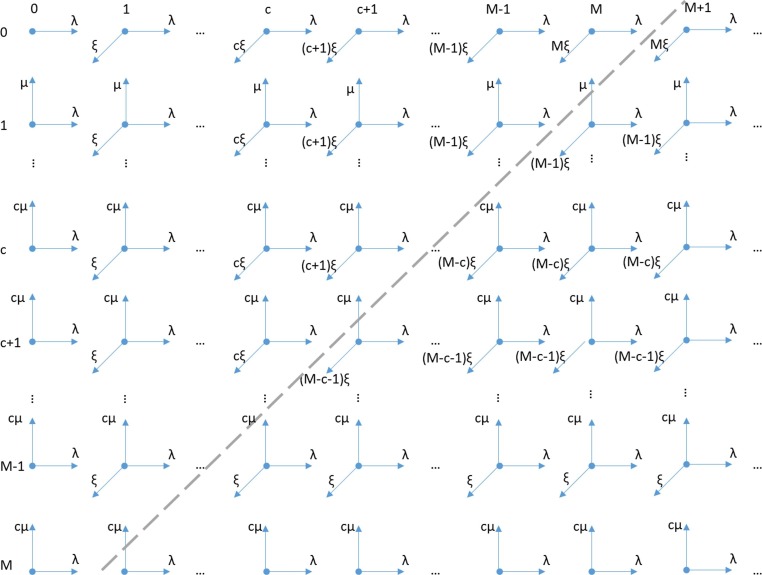
The transition rate from state $(i,j)$ to state $(i+1,j)$ equals the arrival rate λ; the transition rate to state $(i,j-1)$ is $\mathit{\mu }·min(j,c)$ since there are c servers. When $i+j⩽M$, there are i customers in the shopping phase and the transition rate to $(i-1,j+1)$ is $i\xi$. Otherwise, when $i+j>M$, the transition rate from $(i,j)$ to $(i-1,j+1)$ is $(M-j)\xi$ since there are $(M-j)$ customers in the shopping phase. Fig. 1 presents a transition-rate diagram of the M-model system.

Fig. 1.

Transition-rate diagram for the M-model.

The system’s two-dimensional steady-state probabilities are defined as $P_{\mathit{ij}}=P(L_1=i,L_2=j),$ $i=0,1,2,3,...$ $j=0,1,2,...,M$. The probability vectors are defined as ${\overline{P}}_i=((i,0),...,(i,M))$ for $i=0,1,2,...$ where ${\overline{P}}_i$ corresponds to the ith column in the transition-rate diagram. Then, the vector of all system state probabilities, $\overline{P}=({\overline{P}}_0,{\overline{P}}_1,{\overline{P}}_2,...,{\overline{P}}_M,...)$, satisfies

$$\overline{P}Q=\overline{0}$$ (1)

$$\overline{P}·\overline{e}=1$$ (2)

where Q is the so-called infinitesimal generator matrix (see, e.g. Neuts, 1981, p.82; Perlman et al., 2018), $\overline{0}$ is a row vector of zeros, and $\overline{e}$ is a column vector of ones. The generator matrix Q is given by

$$Q=\left(\begin{array}{ccccccccccc}{\text{B}}_{\text{0}}& {\text{A}}_0& 0& & & & & & & & ...\\ {\text{D}}_1& {\text{B}}_1& {\text{A}}_0& 0& & & & & & & ...\\ 0& {\text{D}}_2& {\text{B}}_2& {\text{A}}_0& 0& & & & & & ...\\ & 0& \ddots & \ddots & \ddots & \ddots & & & & & \\ & & \ddots & \ddots & \ddots & \ddots & \ddots & & & & \\ & & & \ddots & {\text{D}}_{M-1}& {\text{B}}_{M-1}& {\text{A}}_0& 0& & & \\ & & & & 0& {\text{D}}_M& {\text{B}}_M& {\text{A}}_0& 0& & \\ & & & & & 0& {\text{A}}_2& {\text{A}}_1& {\text{A}}_0& 0& \\ & & & & & & 0& {\text{A}}_2& {\text{A}}_1& {\text{A}}_0& ...\\ & & & & & & & \ddots & \ddots & \ddots & \ddots \\ & & & & & & & & \ddots & \ddots & \ddots \end{array}\ddots \right)$$

Let ${\text{D}}_i=\left[d_i^{nk}\right]$, $i=1,2,3,...,M$ where $d_i^{nk}$ is the element in column n and row k. Note that only the upper diagonal of ${\text{D}}_i$ has positive elements; all other elements equal zero.

$$d_1^{n+1,n}=\xi n=0,1,2,...,M-1;d_2^{n+1,n}=\left\{\begin{array}{cc}2\xi & n=0,1,2,...,M-2\\ \xi & n=M-1\end{array}\right);$$

$$d_c^{n+1,n}=\left\{\begin{array}{cc}c\xi & n=0,1,2,...,M-c\\ (c-1)\xi & n=M-c-1\\ (c-2)\xi & n=M-c-2\\ ⋮& ⋮\\ \xi & n=M-1\end{array}\right);{\text{and D}}_M={\text{A}}_2$$

Let ${\text{B}}_i=\left[b_i^{nk}\right]=\left[b_{i1}^{nk}\right]+\left[b_{i2}^{nk}\right]$ $i=0,1,2,3,...,M$ where $b_i^{nk}$ is the element in column n and row k. Then,

$$b_{01}^{n,n}=\left\{\begin{array}{cc}-(\mathit{\lambda }+n\mathit{\mu })& n=0,1,2,...,c\\ -(\mathit{\lambda }+c\mathit{\mu })& n=c+1,...,M\end{array}\right),b_{01}^{n,n+1}=\left\{\begin{array}{cc}(n+1)\mathit{\mu }& n=0,1,2,...,c-1\\ c\mathit{\mu }& n=c,c+1,...,M-1\end{array}\right)and{b}_{02}^{n,n}=0$$

while all other elements equal zero.

$$b_{11}^{n,n}=b_{01}^{n,n},b_{11}^{n,n+1}=b_{01}^{n,n+1}and{b}_{12}^{n,n}=\left\{\begin{array}{cc}\xi & n=0,1,2,...,M-1\\ 0& n=M\end{array}\right)$$

and all other elements equal zero;

$$b_{c1}^{n,n}=b_{01}^{n,n},b_{c1}^{n,n+1}=b_{01}^{n,n+1}and{b}_{c2}^{n,n}=\left\{\begin{array}{cc}c\xi & n=0,1,2,...,M-c\\ (c-1)\xi & n=M-c-1\\ (c-2)\xi & n=M-c-2\\ ⋮& ⋮\\ 0& n=M\end{array}\right)$$

all other elements equal zero; and ${\text{B}}_M={\text{A}}_1.$

The matrices A₀, A₁, and A₂ are square matrices of order (M + 1) as follows:

$${\text{A}}_0\text{=}\mathit{\lambda }\text{I}$$

$${\text{A}}_1=\left(\begin{array}{ccccccccc}-(\mathit{\lambda }+M\xi )& & & & & & & & \\ \mathit{\mu }& -(\mathit{\lambda }+(M-1)\xi +\mathit{\mu })& & & & & & & \\ & 2\mathit{\mu }& -(\mathit{\lambda }+(M-2)\xi +\mathit{\mu })& & & & & & \\ & & \ddots & \ddots & & & & & \\ & & & c\mathit{\mu }& -(\lambda +(M-c)\xi +c\mu )& & & & \\ & & & & c\mu & -(\mathit{\lambda }+(M-c-1)\xi +c\mathit{\mu })& & & \\ & & & & & \ddots & \ddots & & \\ & & & & & & c\mathit{\mu }& -(\mathit{\lambda }+\xi +c\mathit{\mu })& \\ & & & & & & & c\mathit{\mu }& -(\mathit{\lambda }+c\mathit{\mu })\end{array}\right)$$

$${\text{A}}_2=\left(\begin{array}{cccccccc}0& M\xi & 0& & & & & \\ & 0& (M-1)\xi & 0& & & & \\ & & \ddots & \ddots & \ddots & & & \\ & & & 0& (M-c)\xi & 0& & \\ & & & & \ddots & \ddots & \ddots & \\ & & & & & 0& 2\xi & 0\\ & & & & & & 0& \xi \\ & & & & & & & 0\end{array}\right)$$

Let $\text{A}={\text{A}}_0+{\text{A}}_1+{\text{A}}_2$. Then,

$$\text{A}=\left(\begin{array}{ccccccccc}-M\xi & M\xi & & & & & & & \\ \mathit{\mu }& -(\mathit{\mu }+(M-1)\xi )& (M-1)\xi & & & & & & \\ & 2\mathit{\mu }& -(2\mathit{\mu }+(M-2)\xi )& (M-2)\xi & & & & & \\ & & \ddots & \ddots & \ddots & & & & \\ & & & c\mathit{\mu }& -(c\mathit{\mu }+(M-c)\xi )& (M-c)\xi & & & \\ & & & & c\mathit{\mu }& -(c\mathit{\mu }+(M-c-1)\xi )& (M-c-1)\xi & & \\ & & & & & \ddots & \ddots & \ddots & \\ & & & & & & c\mathit{\mu }& -(c\mathit{\mu }+\xi )& \xi \\ & & & & & & & c\mathit{\mu }& -c\mathit{\mu }\end{array}\right)$$

Matrix A defines the underlying process of the system, which is depicted in Fig. 2 as a linear Markov process with M + 1 states. In fact, the process defined by A can be considered as a machine repair problem in which $c⩾1$ repairmen maintain $M⩾c$ machines. The lifetime of each machine is exponentially distributed with parameter $\xi$ and the repair time of a machine by a repairman is exponential with $\mathit{\mu }$ intensity. The state of the system is the number of unbroken machines.

Fig. 2.

Transition-rate diagram of A for the M-model.

Denote by $\overline{\mathrm{\Pi }}=({\mathrm{\Pi }}_0,{\mathrm{\Pi }}_1,...,{\mathrm{\Pi }}_M)$ the stationary probability vector satisfying $\overline{\mathrm{\Pi }}\text{A}=\overline{0}$ and $\overline{\mathrm{\Pi }}·\overline{e}=1$.

Proposition 1

The solution of $\overline{\mathrm{\Pi }}\text{A}=\overline{0}$, $\overline{\mathrm{\Pi }}·\overline{e}=1$ is

$${\mathrm{\Pi }}_0={\left[\sum _{k=0}^c\left(\begin{array}{c}M\\ k\end{array}\right){\left(\frac{\xi }{\mathit{\mu }}\right)}^k+\sum _{k=c+1}^M\frac{(M-c)!}{(M-k)!}\frac{1}{c^{k-c}}\left(\begin{array}{c}M\\ c\end{array}\right){\left(\frac{\xi }{\mathit{\mu }}\right)}^k\right]}^{-1}$$

$${\mathrm{\Pi }}_k=\left\{\begin{array}{cc}\left(\begin{array}{c}M\\ k\end{array}\right){\left(\frac{\xi }{\mathit{\mu }}\right)}^k{\mathrm{\Pi }}_0& k=0,1,2,...,c\\ \frac{(M-c)!}{(M-k)!}\frac{1}{c^{k-c}}\left(\begin{array}{c}M\\ c\end{array}\right){\left(\frac{\xi }{\mathit{\mu }}\right)}^k{\mathrm{\Pi }}_0& k=c+1,...,M\end{array}\right)$$

The system stability condition (Neuts, 1981) is $\overline{\mathrm{\Pi }}{\text{A}}_0\overline{e}<\overline{\mathrm{\Pi }}{\text{A}}_2\overline{e}$, and the system is stable if and only if $\mathit{\lambda }<{\sum }_{k=0}^{M-1}{\mathrm{\Pi }}_k(M-k)\xi$.

Next, we explore the stability condition stated in Proposition 1 and provide intuition for the results. In particular, the righthand side of the stability condition approaches $c\mathit{\mu }$ as $\xi$ approaches infinity, and the system then becomes Erlang’s delay queue: an M(λ)/M($\mathit{\mu }$)/c queue with arrival rate λ and c parallel servers who each serve at rate $\mathit{\mu }$. The stability condition is then $\mathit{\lambda }<c\mathit{\mu }.$

As $\mathit{\mu }$ approaches infinity, the mean total service time for each costumer is $1/\xi$ so the system becomes an Erlang’s delay queue with $M$ parallel servers and the stability condition is $\mathit{\lambda }<M\mathit{\xi }$.

Similarly, when M approaches infinity, the shopping phase becomes an M(λ)/M($\xi$)/$\infty$ queue with an output Poisson process (λ). Therefore, the payment phase becomes an M(λ)/M(µ)/c queue and the stability condition is $\mathit{\lambda }<c\mathit{\mu }$. When $c=M,$ each customer who completes shopping goes immediately to the payment phase, and the customer’s mean sojourn time is $\frac{1}{\mu }+\frac{1}{\xi }$. When there are $M=c$ customers in the store, the combined service rate is $\frac{M}{\frac{1}{\mathit{\mu }}+\frac{1}{\xi }}$ and the stability condition is $\frac{M}{\mathit{\lambda }}>\frac{1}{\mathit{\mu }}+\frac{1}{\mathit{\xi }}$. Finally, when there is only a single server (cashier), the right-hand side of the stability condition equals

$$\mathit{RH}{S}_M\equiv \frac{M\mathit{\mu }\mathrm{\Gamma }\left(M,\frac{\mathit{\mu }}{\xi }\right)}{\mathrm{\Gamma }\left(M+1,\frac{\mathit{\mu }}{\xi }\right)}$$

where $\mathrm{\Gamma }(M,z)={\int }_z^{\infty }{e}^{-t}{t}^{(M-1)}dt$ is the incomplete Gamma function.

As in Neuts (1981), a rate matrix R exists that satisfies

$${\mathrm{A}}_0+{\mathrm{R}\mathrm{A}}_1+{\mathrm{R}}^2{\mathrm{A}}_2=0$$ (3)

while the probability vectors satisfy

$${\overline{P}}_{M+k}={\overline{P}}_M{\text{R}}^{k}k=0,1,2,\dots .$$ (4)

R is the minimal non-negative solution of Eq. (3) and is usually calculated numerically via a successive substitution algorithm (see, e.g., Harchol-Balter, 2013). See Hanukov and Yechiali (2020) for cases in which matrix R can be expressed explicitly.

By Eqs. (1), (2), the balance equations are

$${\overline{P}}_0{\text{B}}_{\text{0}}+{\overline{P}}_1{\text{D}}_{\text{1}}=\overline{0}$$ (5)

$${\overline{\text{P}}}_{j-1}{\text{A}}_{\text{0}}+{\overline{\text{P}}}_j{\text{B}}_{\text{j}}+{\overline{\text{P}}}_{j+1}{\text{D}}_{\text{j + 1}}=\overline{0}j=1,2,...,M-1$$ (6)

$$\sum _{j=0}^{\infty }{\overline{P}}_j\overline{e}=\sum _{j=0}^{M-1}{\overline{P}}_j\overline{e}+{\overline{P}}_M{\left[I-R\right]}^{-1}\overline{e}=1$$ (7)

The $M+1$ Eqs. (5), (6), (7) uniquely determine the boundary probability vectors ${\overline{P}}_0,{\overline{P}}_1,{\overline{P}}_2,...,{\overline{P}}_M$.

2.2. Risk of infection

Since the risk of infection increases as the number of customers in a store increases, we estimate the risk of infection as proportional to $\text{E}\left[L(L-1)\right]$. That is, when L customers are present in the store, each one can be infected by the other $L-1$ customers. Also, the risk of infection is lower in more-open areas and could depend on whether social distance can be and is maintained. Therefore, in this section we calculate the combined risk of infection for customers along their waiting, shopping, and payment routes (phases). Let L ₁ ^SHOP denote the number of shoppers and let L ₁ ^OUT denote the number of customers lining up outside the store with L ₁ = L ₁ ^SHOP + L ₁ ^OUT. We start by calculating $\text{E}\left[L_1\right]$.

$$\text{E}\left[L_1\right]=\sum _{i=0}^{\infty }i{\overline{P}}_i·\overline{e}=\sum _{i=0}^{M-1}i{\overline{P}}_i·\overline{e}+{\overline{P}}_M\sum _{i=M}^{\infty }i{R}^{i-M}\overline{e}=\sum _{i=0}^{M-1}i{\overline{P}}_i·\overline{e}+{\overline{P}}_M\left[(M-1){\left[I-R\right]}^{-1}+{\left[I-R\right]}^{-2}\right]\overline{e}$$ (8)

The risk to shoppers of being infected is considered proportional to $\text{E}\left[L_1^{\mathit{SHOP}}(L_1^{\mathit{SHOP}}-1)\right]$. The risk of customers waiting outside the store is proportional to $\left[L_1^{\mathit{OUT}}(L_1^{\mathit{OUT}}-1)\right]$.

Proposition 2

Let

$${\overline{g}}_i=\left(\underset{M-i+1}{\underbrace{i,i,i,...,i}},\underset{i}{\underbrace{i-1,i-2,...,1,0}}\right),i=0,1,...,M;{\overline{g}}_i={\overline{g}}_{M}i>M$$

$$\overline{g_i^2}=\left(\underset{M-i+1}{\underbrace{i^2,i^2,i^2,...,i^2}},\underset{i}{\underbrace{{(i-1)}^2,{(i-2)}^2,...,1,0}}\right),i=0,1,...,M;\overline{g_i^2}=\overline{g_M^2}i>M$$

$${\overline{v}}_i=\left\{\begin{array}{cc}\left(\underset{M-i+1}{\underbrace{0,0,0,...,0}},\underset{i}{\underbrace{1,2,3,...,i}}\right)& i=0,1,2,...,M\\ \left(i-M,i-M+1,...,i\right)& i=M+1,...\end{array}\text{and}\right)$$

$$\overline{v_i^2}=\left\{\begin{array}{cc}\left(\underset{M-i+1}{\underbrace{0,0,0,...,0}},\underset{i}{\underbrace{1,2^2,3^2,...,i^2}}\right)& i=0,1,2,...,M\\ \left({(i-M)}^2,{(i-M+1)}^2,...,i^2\right)& i=M+1,...\end{array}\right)$$

be four sets of column vectors, each of size $\left(M+1\right)$. Then,

• i. $\text{E}\left[L_1^{\mathit{SHOP}}\right]={\sum }_{i=0}^{M-1}{\overline{P}}_i{\overline{g}}_i+{\sum }_{i=M}^{\infty }{\overline{P}}_i{\overline{g}}_M={\sum }_{i=0}^{M-1}{\overline{P}}_i{\overline{g}}_i+{\overline{P}}_M{\sum }_{i=M}^{\infty }{R}^{i-M}{\overline{g}}_M={\sum }_{i=0}^{M-1}{\overline{P}}_i{\overline{g}}_i+{\overline{P}}_M{[I-R]}^{-1}{\overline{g}}_M$.
• ii. $\text{E}\left[{(L_1^{\mathit{SHOP}})}^2\right]={\sum }_{i=0}^{\infty }{\overline{P}}_i\overline{g_i^2}={\sum }_{i=0}^{M-1}{\overline{P}}_i\overline{g_i^2}+{\overline{P}}_M{\sum }_{i=M}^{\infty }{R}^{i-M}\overline{g_M^2}={\sum }_{i=0}^{M-1}{\overline{P}}_i\overline{g_i^2}+{\overline{P}}_M{[I-R]}^{-1}\overline{g_M^2}$.
• iii. $\text{E}\left[L_1^{\mathit{OUT}}\right]=\text{E}\left[L_1^{}\right]-\text{E}\left[L_1^{\mathit{SHOP}}\right]$.
• iv. $\text{E}\left[{\left(L_1^{\mathit{OUT}}\right)}^2\right]={\sum }_{i=0}^{\infty }{\overline{P}}_i\overline{v_i^2}$.

Proof

In the case $L_1=i\text{and}{L}_2=j$ such that $i+j⩽M,$ there are i customers in the shopping phase, j customers in the payment phase, and no customers waiting outside the store. In the case $i+j>M,$ there are $i+j-M$ customers waiting outside since only M customers are allowed inside. Since there are j customers in the payment phase, $M-j$ customers are in the shopping phase. □

Similarly, the risk of customers in the payment phase is proportional to $\text{E}\left[L_2^{\mathit{PAY}}(L_2^{\mathit{PAY}}-1)\right]$.

Proposition 3

Let $\overline{z}=\left(0,1,2,...,c,...,M\right),\overline{z^2}=\left(0,1,2^2,...,c^2,...,M^2\right)$ be two column vectors each of size (M + 1). Then,

• i. $\text{E}\left[L_2^{\mathit{PAY}}\right]=\left({\sum }_{i=0}^{\infty }{\overline{P}}_i\right)\overline{z}=\left({\sum }_{i=0}^{M-1}{\overline{P}}_i\right)\overline{z}+\left({\sum }_{i=M}^{\infty }{\overline{P}}_i\right)\overline{z}=\left({\sum }_{i=0}^{M-1}{\overline{P}}_i+{\overline{P}}_M{\left[I-R\right]}^{-1}\right)\overline{z}$.
• ii. $\text{E}\left[{(L_2^{\mathit{PAY}})}^2\right]=\left({\sum }_{i=0}^{\infty }{\overline{P}}_i\right)\overline{z^2}=\left({\sum }_{i=0}^{M-1}{\overline{P}}_i\right)\overline{z^2}+\left({\sum }_{i=M}^{\infty }{\overline{P}}_i\right)\overline{z^2}=\left({\sum }_{i=0}^{M-1}{\overline{P}}_i+{\overline{P}}_M{\left[I-R\right]}^{-1}\right)\overline{z^2}$.

When the system is stable, the mean rate of arrival rate at the shopping phase is $\mathit{\lambda }$. Similarly, the mean rate of arrival at the payment phase is also $\mathit{\lambda }$. Applying Little’s Law, one can calculate the mean waiting times:

$$\text{E}\left[W^{\mathit{SHOP}}\right]=\frac{\text{E}\left[L_1^{\mathit{SHOP}}\right]}{\lambda }\text{E}\left[W^{\mathit{OUT}}\right]=\frac{\text{E}\left[L_1^{\mathit{OUT}}\right]}{\lambda }\text{and}\text{E}\left[W^{\mathit{PAY}}\right]=\frac{\text{E}\left[L_2^{\mathit{PAY}}\right]}{\lambda }.$$

3. The NM-model: Maximum number of customers at the cashier area and shopping inside the store

3.1. Model description, formulation, and analysis

We now model a setting in which the store sets aside a separate waiting space near the cashiers for at most N ≥ 0 customers in the payment phase and those customers wait in a single line in the designated area (if necessary) to be admitted by the next free cashier. As in the M-model, the authorities in this model have imposed a limit, M, on the total number of customers allowed inside the store. Thus, in this setting, the store is divided into two separate areas: (i) the payment area with c ≥ 1 parallel cashiers and waiting space of size N customers and (ii) the shopping area, in which the maximum number of customers allowed, K. Thus, the maximum number of customers is the store is $M=c+N+K$.

In this model, a customer first spends a random period of time in the shopping phase/area that is exponentially distributed with mean 1/ξ and then proceeds to the payment phase/area. When there are exactly c + N payers, this customer “orbits” in the shopping area for another exponentially distributed period of time with the same mean 1/ξ (see, e.g., Avrachenkov et al., 2014, Perel and Yechiali, 2014). Otherwise, when the number of customers in the cashier area is less than c + N, the customer enters the cashier area and becomes a payer. When at least one of the cashiers is not busy, the payer proceeds directly to a cashier and pays. As in the M-model, the payment (service) duration is exponentially distributed with mean 1/µ. All shopping, service, and orbit times are independent of each other and independent of the arrival process.

Let L ₁ ^SHOP denote the number of customers in the shopping area and let L ₁ ^OUT denote the number of customers lining up outside the store. Let L ₁ = L ₁ ^SHOP + L ₁ ^OUT. Let L ₂ denote the number of customers in the cashier area. Then, the system’s state-space is

$$S=\left\{(L_1,L_2)=(i,j):i=0,1,2,3,...;j=0,1,2,3,...,c+N\right\}$$

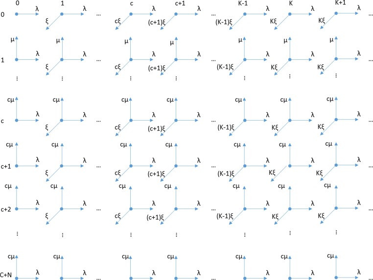
The transition-rate diagram for this system is depicted in Fig. 3 .

Fig. 3.

Transition-rate diagram for the NM-model.

The system’s two-dimensional steady-state probabilities are defined as $P_{\mathit{ij}}=P(L_1=i,L_2=j),$ $i=0,1,2,3,...$; $j=0,1,2,...,c+N.$ The states are then arranged in a lexicographic order such that the state space is

$$S=\left\{(0,0),(0,1),(0,2),...,(0,c),(0,c+1),...,(0,c+N);(1,0),(1,1),(1,2),...,(1,c),(1,c+)...(1,c+N);..\right).$$

$$\left(...;(i,0),(i,1),(i,2),...,(i,c),(i,c+)...(i,c+N);...\right\}$$

The probability vectors are defined as ${\overline{P}}_i=((i,0),...,(i,c+N))$ for $i=0,1,2,...$ where ${\overline{P}}_i$ corresponds to the ith column in the transition-rate diagram. Then, the vector of all of the system state probabilities, $\overline{P}=({\overline{P}}_0,{\overline{P}}_1,{\overline{P}}_2,...,{\overline{P}}_K,...)$, satisfies Eqs. (1), (2) where the generator matrix Q is given by

$$Q=\left(\begin{array}{ccccccccccc}{\text{B}}_{\text{0}}& {\text{A}}_0& 0& & & & & & & & ...\\ {\text{D}}_1& {\text{B}}_1& {\text{A}}_0& 0& & & & & & & ...\\ 0& {\text{D}}_2& {\text{B}}_2& {\text{A}}_0& 0& & & & & & ...\\ & 0& \ddots & \ddots & \ddots & \ddots & & & & & \\ & & \ddots & \ddots & \ddots & \ddots & \ddots & & & & \\ & & & \ddots & {\text{D}}_{K-1}& {\text{B}}_{K-1}& {\text{A}}_0& 0& & & \\ & & & & 0& {\text{D}}_K& {\text{B}}_K& {\text{A}}_0& 0& & \\ & & & & & 0& {\text{A}}_2& {\text{A}}_1& {\text{A}}_0& 0& \\ & & & & & & 0& {\text{A}}_2& {\text{A}}_1& {\text{A}}_0& ...\\ & & & & & & & \ddots & \ddots & \ddots & \ddots \\ & & & & & & & & \ddots & \ddots & \ddots \end{array}\ddots \right)$$

where

$${\text{D}}_i=\left(\begin{array}{ccccccc}0& i\xi & & & & & \\ & 0& i\xi & & & & \\ & & \ddots & \ddots & \ddots & & \\ & & & & & & \\ & & & & & i\xi & \\ & & & & & 0& i\xi \\ & & & & & & 0\end{array}\right)i=1,2,3,...,K$$

$${\text{B}}_j=\left(\begin{array}{ccccccc}-(\mathit{\lambda }+j\xi )& & & & & & \\ \mathit{\mu }& -(\mathit{\lambda }+j\xi +\mathit{\mu })& & & & & \\ & 2\mathit{\mu }& -(\mathit{\lambda }+j\xi +2\mathit{\mu })& & & & \\ & & \ddots & \ddots & & & \\ & & & c\mathit{\mu }& -(\mathit{\lambda }+j\xi +c\mathit{\mu })& & \\ & & & & \ddots & \ddots & \\ & & & & & c\mathit{\mu }& -(\mathit{\lambda }+c\mathit{\mu })\end{array}\right)j=0,1,2,3,\dots ,K,$$

${\text{A}}_0\text{=}\lambda \text{I}$, ${\text{A}}_{\text{1}}{\text{= B}}_{\text{K}}$, and ${\text{A}}_{\text{2}}{\text{= D}}_{\text{K}}$. The matrix A₀ and all square matrices B_j and B_i are of order (c + N + 1). Again, there exists a rate matrix R that satisfies

$${\mathrm{A}}_0+{\mathrm{R}\mathrm{A}}_1+{\mathrm{R}}^2{\mathrm{A}}_2=0$$ (9)

where the probability vectors satisfy

$${\overline{P}}_{K-1+i}={\overline{P}}_{K-1}{R}^{i}i=0,1,2,....$$ (10)

Combining Eqs. (2), (10), we obtain

$$\overline{P}·\overline{e}=\sum _{i=0}^{K-1}{\overline{P}}_i·\overline{e}+{\overline{P}}_K{\left[I-R\right]}^{-1}·\overline{e}=1.$$ (11)

The first K equations of Eq. (1) are

$${\overline{P}}_0{\text{B}}_{\text{0}}+{\overline{P}}_1{\text{D}}_{\text{1}}=\overline{0}$$ (12)

$${\overline{\text{P}}}_{j-1}{\text{A}}_{\text{0}}+{\overline{\text{P}}}_j{\text{B}}_{\text{j}}+{\overline{\text{P}}}_{j+1}{\text{D}}_{\text{j + 1}}=\overline{0}j=1,2,3,...,K-1$$ (13)

Eqs. (12), (13) yield the boundary probability vectors (${\overline{P}}_0,{\overline{P}}_1,{\overline{P}}_2,...,{\overline{P}}_K$) needed for calculation of the performance measures in the sequel.

Let $\text{A}={\text{A}}_0+{\text{A}}_1+{\text{A}}_2$. Then,

$$A=\left(\begin{array}{ccccccccccc}-K\xi & K\xi & & & & & & & & & \\ \mathit{\mu }& -(\mathit{\mu }+K\xi )& K\xi & & & & & & & & \\ & 2\mathit{\mu }& -(2\mathit{\mu }+K\xi )& K\xi & & & & & & & \\ & & \ddots & \ddots & \ddots & & & & & & \\ & & & \ddots & \ddots & \ddots & & & & & \\ & & & & c\mathit{\mu }& -(c\mathit{\mu }+K\xi )& K\xi & & & & \\ & & & & & c\mathit{\mu }& -(c\mathit{\mu }+K\xi )& K\xi & & & \\ & & & & & & \ddots & \ddots & \ddots & & \\ & & & & & & & \ddots & \ddots & \ddots & \\ & & & & & & & & c\mathit{\mu }& -(c\mathit{\mu }+K\xi )& K\xi \\ & & & & & & & & & c\mathit{\mu }& -c\mathit{\mu }\end{array}\right)$$

The matrix A defining the underlying process of this system is equivalent to a truncated Erlang’s model of Poisson arrival with rate $K\xi$, c parallel exponential servers each with rate µ, and an additional waiting buffer of size N. Fig. 4 presents its transition-rate diagram.

Proposition 5

Let $a=\frac{K\xi }{\mathit{\mu }}$, $\rho =\frac{K\xi }{c\mathit{\mu }}$. The system is stable if and only if

$$\mathit{\lambda }<K\xi \left(1-\frac{a^c}{c!}{\mathit{\rho }}^N{\left(\sum _{i=0}^{c-1}\frac{a^i}{i!}+\frac{a^c}{c!}\frac{1-{\mathit{\rho }}^{N+1}}{1-\mathit{\rho }}\right)}^{-1}\right)$$

Proof

Matrix A has a stationary probability vector $\overline{\mathrm{\Pi }}=({\mathrm{\Pi }}_0,{\mathrm{\Pi }}_1,...,{\mathrm{\Pi }}_c,...,{\mathrm{\Pi }}_{c+N})$ that satisfies $\overline{\mathrm{\Pi }}\text{A}=\overline{0}$ and $\overline{\mathrm{\Pi }}·\overline{e}=1$. Then, ${\mathrm{\Pi }}_i=\frac{a^i}{i!}{\mathrm{\Pi }}_{0}i=1,2,...,c.$, ${\mathrm{\Pi }}_{c+n}={\mathrm{\Pi }}_c{\mathit{\rho }}^{n}n=0,1,2,...,N$, and ${\mathrm{\Pi }}_0={\left[{\sum }_{i=0}^{c-1}\frac{a^i}{i!}+\frac{a^c}{c!}\frac{1-{\mathit{\rho }}^{N+1}}{1-\mathit{\rho }}\right]}^{-1}$. The stability condition is given by Neuts (1981) as $\overline{\mathrm{\Pi }}{\text{A}}_0\overline{e}<\overline{\mathrm{\Pi }}{\text{A}}_2\overline{e},$ which translates into $\mathit{\lambda }<K\xi (1-{\mathrm{\Pi }}_{c+N})=K\xi \left(1-\frac{a^c}{c!}{\mathit{\rho }}^N{\mathrm{\Pi }}_0\right).$ □

Fig. 4.

Transition-rate diagram of A for the NM-model.

Set $\mathit{RH}{S}_{\mathit{NM}}\equiv K\xi \left(1-\frac{a^c}{c!}{\mathit{\rho }}^N{\left({\sum }_{i=0}^{c-1}\frac{a^i}{i!}+\frac{a^c}{c!}\frac{1-{\mathit{\rho }}^{N+1}}{1-\mathit{\rho }}\right)}^{-1}\right)$. Corollary 1 specifies the value of $\mathit{RH}{S}_{\mathit{NM}}$ for some special cases.

Corollary 1

• (i) $\underset{c\to \infty }{lim}RH{S}_{\mathit{NM}}=K\xi .$
• (ii) When $N=0,$ $\mathit{RH}{S}_{\mathit{NM}}=K\xi \frac{{\sum }_{i=0}^{c-1}\frac{a^i}{i!}}{{\sum }_{i=0}^c\frac{a^i}{i!}}=\frac{cK\xi \mathrm{\Gamma }\left(c,\frac{K\xi }{\mu }\right)}{\mathrm{\Gamma }\left(c+1,\frac{K\xi }{\mu }\right)}$. In particular, when N = 0 and c = 1, $\mathit{RH}{S}_{\mathit{NM}}=\frac{1}{\frac{1}{\mathit{\mu }}+\frac{1}{K\xi }}$.
• (iii) $\underset{\xi \to \infty }{lim}RH{S}_{\mathit{NM}}=c\mathit{\mu }.$
• (iv) $\underset{\mu \to \infty }{lim}RH{S}_{\mathit{NM}}=K\xi .$

It follows from Corollary 1(i) that, when the number of cashiers is infinitely large, only the shopping area determines the stability of the system. As such, the shopping area is a classical Erlang’s delay model with Poisson arrival rate $\mathit{\lambda }$ and $K$ parallel servers, each with rate $\xi$, and the stability condition is $\mathit{\lambda }<K\xi$. When $N=0,$ the right-hand side of the stability condition can be written explicitly or with the aid of the incomplete Gamma function (see Corollary 1(ii)). For the special case in which $N=0$ and $c=1$, the combined service rate when there are K shoppers is Kξ. Thus the stability condition is $\frac{1}{\mathit{\lambda }}>\frac{1}{\mathit{\mu }}+\frac{1}{K\xi }$. It follows from Corollary 1(iii) that, when $\xi$ is infinitely large, customers do not spend time in the shopping area and move immediately to the payment area. Therefore, the system is reduced to a classical M/M/c queue with stability condition $\mathit{\lambda }<c\mathit{\mu }$. Finally, when $\mathit{\mu }$ approaches infinity, the system becomes the M $(\mathit{\lambda })$/M $(\xi )$/K queue with stability condition $\lambda <K\xi$ (Corollary 1(iv)).

3.2. Risk of infection

As in the M-model, the risk of customers being infected at each area is estimated as $\text{E}\left[{(L_1^{\mathit{OUT}})}^2\right]-\text{E}\left[L_1^{\mathit{OUT}}\right],\text{E}\left[{(L_1^{\mathit{SHOP}})}^2\right]-\text{E}\left[L_1^{\mathit{SHOP}}\right]\text{and}\text{E}\left[{(L_2^{\mathit{PAY}})}^2\right]-\text{E}\left[L_2^{\mathit{PAY}}\right]$, respectively. The following proposition shows how these measures are calculated.

Proposition 5

Let $\overline{u}=\left(0,1,2,...,c,...,c+N\right)\text{and}\overline{u^2}=\left(0,1,2^2,...,c^2,...,{(c+N)}^2\right)$ be two column vectors, each of size $\left(c+N+1\right)$. Then,

• i. $\text{E}\left[L_1^{\mathit{OUT}}\right]={\overline{P}}_K\left({\left[I-R\right]}^{-2}-{\left[I-R\right]}^{-1}\right)·\overline{e}$.
• ii. $\text{E}\left[{(L_1^{\mathit{OUT}})}^2\right]={\sum }_{i=K+1}^{\infty }{(i-K)}^2{\overline{P}}_i·\overline{e}$.
• iii. $\text{E}\left[L_1^{\mathit{SHOP}}\right]={\sum }_{i=0}^{K}i{\overline{P}}_i·\overline{e}+K\left(1-{\sum }_{j=0}^K{\overline{P}}_j·\overline{e}\right)$.
• iv. $\text{E}\left[{(L_1^{\mathit{SHOP}})}^2\right]={\sum }_{i=0}^K{i}^2{\overline{P}}_i·\overline{e}+K^2\left(1-{\sum }_{j=0}^K{\overline{P}}_j·\overline{e}\right)$.
• v. $\text{E}\left[L_2^{\mathit{PAY}}\right]=\left({\sum }_{i=0}^{K-1}{\overline{P}}_i+{\overline{P}}_K{\left[I-R\right]}^{-1}\right)\overline{u}$.
• vi. $\text{E}\left[{(L_2^{\mathit{PAY}})}^2\right]=\left({\sum }_{i=0}^{K-1}{\overline{P}}_i+{\overline{P}}_K{\left[I-R\right]}^{-1}\right)\overline{u^2}$.

Proof

• (i) $\text{E}\left[L_1^{\mathit{OUT}}\right]={\sum }_{i=1}^{\infty }\mathit{iP}(L_1=K+i)={\overline{P}}_K{\sum }_{i=1}^{\infty }i{R}^i·\overline{e}={\overline{P}}_K\left({\left[I-R\right]}^{-2}-{\left[I-R\right]}^{-1}\right)·\overline{e}$.

• (iii) $\text{E}\left[L_1^{\mathit{SHOP}}\right]={\sum }_{i=0}^K\mathit{iP}(L_1=i)+K{\sum }_{m=1}^{\infty }P(L_1=K+m)={\sum }_{i=0}^{K}i{\overline{P}}_i·\overline{e}+K\left(1-{\sum }_{i=0}^K{\overline{P}}_i·\overline{e}\right).$

• Similar to the proof of Proposition 3. □

Again, if the system is stable, the mean rate of arrival to the shopping area is $\mathit{\lambda }$. Similarly, the mean rate of arrival to the cashier area is also $\mathit{\lambda }$. Applying Little’s Law, the mean waiting time outside the store is $\text{E}\left[W^{\mathit{OUT}}\right]=\frac{\text{E}\left[L_{\text{1}}^{\mathit{OUT}}\right]}{\mathit{\lambda }}=\frac{{\overline{P}}_M\left({\left[I-R\right]}^{-2}-{\left[I-R\right]}^{-1}\right)·\overline{e}}{\mathit{\lambda }}$. The mean waiting time at the shopping area is $\text{E}\left[W^{\mathit{SHOP}}\right]=\frac{\text{E}\left[L_{\text{1}}^{\mathit{SHOP}}\right]}{\mathit{\lambda }}$ and the mean waiting time at the payer area is $\text{E}\left[W^{\mathit{PAY}}\right]=\frac{\text{E}\left[L_2^{\mathit{PAY}}\right]}{\mathit{\lambda }}.$

4. Sensitivity analysis

We next study the effect of the two models’ parameters on the performance measures. Let the arrival rate, service rate, and shopping rate, respectively, be $\mathit{\lambda }=18,\mathit{\mu }=10,\text{and}\xi =3$ customers per hour. Set M = 15, N = 5, and c = 2 so that the maximum number of customers in the shopping area is $K=15-5-2=8.$ For these values, the right-hand side of the stability condition is $\mathit{RH}{S}_M=\text{19.927}$ in the M-model and $\mathit{RH}{S}_{\mathit{NM}}=18.625$ in the NM-model. Note that $\mathit{RH}{S}_{\mathit{NM}}<RH{S}_M$ since there are additional restrictions on the NM-model.

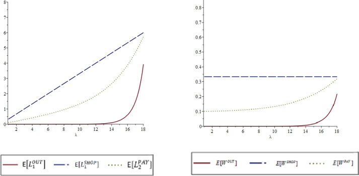
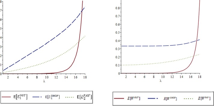
When we change the arrival rate $\mathit{\lambda }$ from 0 to 18, the mean number of customers and corresponding mean waiting times for customers, respectively, are $E[L_1^{\mathit{OUT}}]\text{and}E[W^{\mathit{OUT}}]$ outside the store, $(E[L_1^{\mathit{SHOP}}],E[W^{\mathit{SHOP}}])$ at the shopping area, and $(E[L_2^{\mathit{PAY}}],E[W^{\mathit{PAY}}])$ at the cashier area, as depicted in Figs. 5 and 6.

Fig. 5.

Effect of arrival rate (λ) on performance measures for the M-model.

Fig. 6.

Effect of arrival rate (λ) on performance measures for the NM-model.

Figs. 5 and 6 show that there are no differences in the values of the performance measures under the two models for outside the store, in the shopping area, and in the payment area when the system is not congested (i.e., $\mathit{\lambda }<<RH{S}_{\mathit{NM}}<RH{S}_M$). That is, for small values of $\mathit{\lambda }$ in uncongested systems, almost no customers wait outside the store, customers complete the shopping phase after an average of $1/\xi$ units of time, and the mean waiting times (sojourn) for payers is about $1/\mathit{\mu }$. However, when the system is congested, the two model performance measures behave differently. The number of customers waiting outside the store increases more rapidly under the NM-model than under the M-model. As a result, both the number of customers waiting outside and their mean waiting times are greater under the NM-model. The mean waiting times in the shopping phase under the M-model equals $1/\xi$ since leaving the shopping area is never delayed. However, under the NM-model (Fig. 6 ), which has a limit on the number of customers who can wait in the payment area (N = 5), some customers have to delay leaving the shopping area because the payment waiting space is full. Thus, both the number of shoppers and their mean waiting times are greater under the NM-model. The mean number of payers and their mean waiting times are lower in the NM-model than in the M-model because only a limited number of payers, $c+N⩽M,$ are allowed in the payment area under the NM-model.

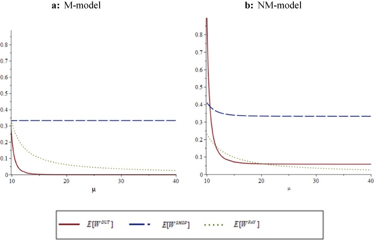
Fig. 7 shows the results of a change in the cashier service rate on the three mean waiting times for the M-model (7a) and NM-model (7b). Note that the minimal value of $\mathit{\mu }$ that maintains the stability conditions is 10. Hence, we study the effect of increasing the service rate up to $\mathit{\mu }=40$.

Fig. 7.

Effect of cashier service rate (µ) on expected waiting times.

We find that increasing the service rate has no impact on mean waiting time in the shopping phase under the M-model since no restrictions are placed on shopping time in that case and shopping mean waiting time equals $1/\xi .$ However, when the system under the NM-model is congested, the mean waiting times for shoppers is greater than $1/\xi$. Again, this result follows since there is a limit on the number of payers allowed in the payment waiting area, causing some shoppers to have to orbit in the shopping area (they are in the payment phase but must remain in the shopping area). As the service rate increases, mean waiting times for payers and customers outside the store clearly decrease. Under both models, as $\mathit{\mu }$ increases, payer mean waiting times approaches $E[W^{\mathit{PAY}}]=1/\mathit{\mu }$ since fewer and fewer customers have to wait in line in the payment area. For outside customers, the mean waiting times reduces to zero as $\mathit{\mu }$ increases under the M-model and reaches a positive limit under the NM-model. This follows since, in the NM-model, the total number of customers inside the store is rigidly assigned to two separate areas, reducing the efficiency of the system.

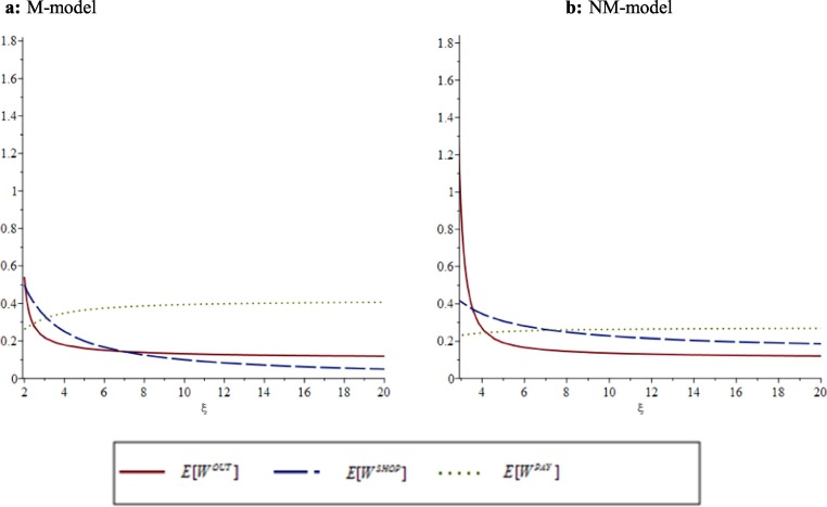
The impacts of changing the time spent shopping ($\xi$) on the respective mean waiting times for the M-model and NM-model are depicted in Fig. 8 . The smallest value of $\xi$ for which the system is stable is 2 in the M-model and 3 in the NM-model.

Fig. 8.

Effect of mean shopping time ($\xi$) on expected waiting times.

As previously noted, the mean waiting times for shoppers equals $1/\xi$ under the M-model and is greater under the NM-model because of restriction in the payment area. When increasing $\xi$, the mean waiting times of outside customers in both models approaches a limit that depends on the other model parameters. The mean payer wait time approaches 0.416 under the M-model and 0.27 under the NM-model. This follows since only N customers are allowed to wait at the payment area under the NM-model; under the M-model, up to M  –  c customers can wait there to be served by cashiers. The mean waiting times of customers outside approaches a positive limit since a queue is forming at the cashier area, which delays permission for new customers to enter the store.

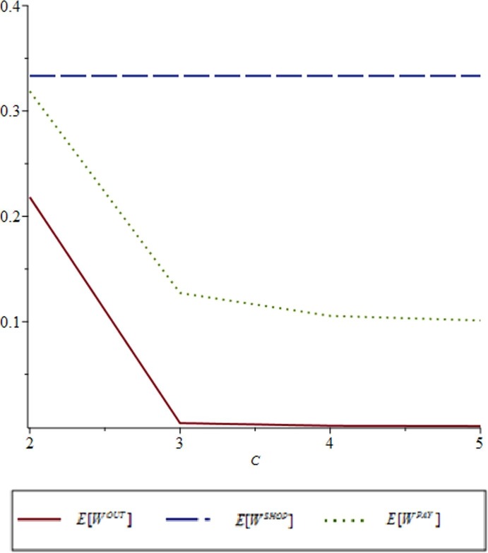
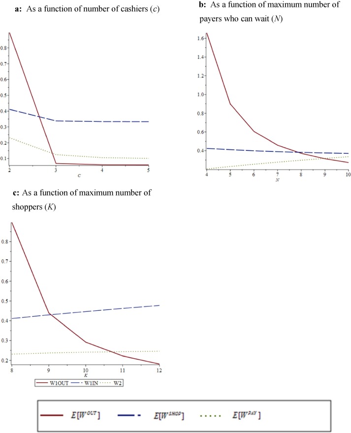
The effect of the number of cashiers and of the maximum number of customers in the store on mean waiting times is depicted in Figs. 9 and 10. The minimal values of c that maintain the stability conditions are 2. Thus, we examine values of $c\in \left\{2,3,4,5\right\}$. Changing the number of cashiers, as expected, has no impact on shoppers’ expected wait time. However, under the M-model, an increase in the number of cashiers from 2 to 3 decreases the arrival ratio $\mathit{\lambda }/\mathit{RH}{S}_M$ from $18/19.9=93\%$ to 18/28.2 = 63%, and when $c=4$, the arrival ratio is $\mathit{\lambda }/\mathit{RH}{S}_M=55\%.$ Thus, adding one cashier (moving from $c=2$ to $c=3$) has a major impact on the mean waiting time of customers outside the store – the outside wait time becomes almost negligible – and a major impact on the mean payer wait time. When $c=4$, almost no customers wait outside the store and the mean payer wait time approaches $E[W^{\mathit{PAY}}]=1/\mathit{\mu }$.

Fig. 9.

Effect of number of cashiers (c) on expected waiting times for the M-model.

Fig. 10.

Effect of number of customers allowed in the store (M) on expected waiting times for the M-model.

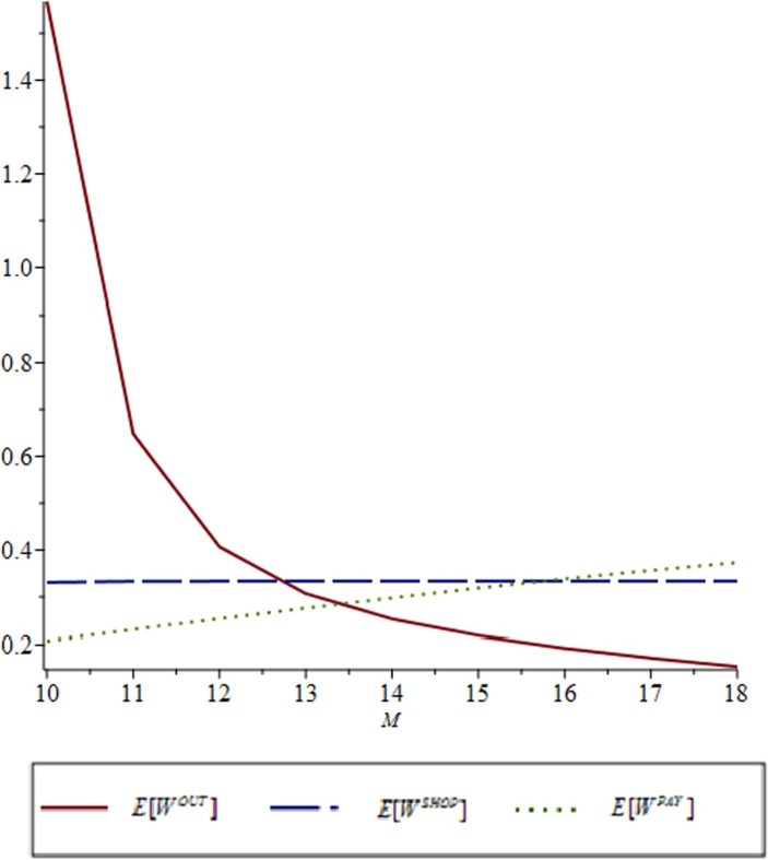
Under the M-model, the minimal value of the number of customers in the store that maintains the stability condition is M = 10. Thus, we let $M\in \left\{10,11,...,18\right\}$. As depicted in Fig. 10, changing the value of M has no impact on shopper waiting time since, when the system is stable, the mean number of shoppers is $\mathit{\lambda }/\xi$ and $E[W^{\mathit{SHOP}}]=1/\xi .$ Increasing the number of customers allowed in the store clearly reduces $E[W^{\mathit{OUT}}]$ and increases $E[W^{\mathit{PAY}}].$

Remember that the store in the NM-model is divided into separate shopping and payment areas, both of which are restricted in terms of the number of customers who can occupy those spaces. The shopping area is limited to K customers and the payment area at the cashier space is limited to $c+N$ customers. Thus, increasing the value of c, N, or K (see Fig. 11) increases the value of the maximum number of customers who can be in the store $(M=c+N+K).$

Fig. 11.

Expected waiting times under the NM-model.

As in the M-model (Fig. 9 ), increasing the number of cashiers (c) in the NM-model results in a diminishing reduction in mean waiting times of customers lining up outside and of payers. That is, as c increases, $E[W^{\mathit{OUT}}]$ approaches zero and $E[W^{\mathit{PAY}}]$ approaches $1/\mathit{\mu }$. However, increasing c under the NM-model also reduces $E[W^{\mathit{SHOP}}]$ since a greater number of cashiers increases the service rate at the payment area. Customers can proceed more rapidly through the payment phase, reducing the amount of time spent waiting in the designated area and reducing the number of customers who must orbit in the shopping area.

The smallest value of N (the number of payers who can occupy the payment space) that sustains the stability condition is 4. When the value of N increases, as depicted in Fig. 11b, the system becomes less congested, and $E[W^{\mathit{OUT}}]$ decreases and approaches zero when N is relatively large greater number of customers are allowed inside the store). Similarly, $E[W^{\mathit{SHOP}}]$ decreases and approaches $1/\xi .$ As expected, increasing the size of the payment waiting area increases $E[W^{\mathit{PAY}}]$.

Increasing the allowed number of customers in the shopping phase (K) increases both $E[W^{\mathit{SHOP}}]$ and $E[W^{\mathit{PAY}}]$. The system becomes more congested and greater values of K increase the rate of arrival at the payment area because the number of customers in the shopping area increases. Clearly, increasing K increases the total number of shoppers in the store, thus reducing $E[W^{\mathit{OUT}}].$

5. The COVID-19 queueing game

Several studies have adopted game-theoretic approaches when analyzing safety-related events (see Winkler et al. (2019) for a review). We construct and analyze a COVID-19 queueing game between the authority aiming to reduce the risk of infection while keeping customers and workers safe and a businesses that wants to minimize its costs. Specifically, the authority chooses the maximum number of customers allowed in the store, M. The objective of the authority is

$$\text{A}\equiv min\left\{{\mathit{\alpha }}_1\text{E}\left[L_1^{\mathit{OUT}}(L_1^{\mathit{OUT}}-1)\right]+{\mathit{\alpha }}_2\text{E}\left[L_1^{\mathit{SHOP}}(L_1^{\mathit{SHOP}}-1)\right]+{\mathit{\alpha }}_3\text{E}\left[L_{\text{2}}^{\mathit{Pay}}(L_2^{\mathit{Pay}}-1)\right]\right\}$$ (14)

where ${\mathit{\alpha }}_i$ denotes the weight the authority assigns to each measure of risk. It is reasonable to assume that the authority assigns a smaller weight to queues forming outside a store; therefore, in this case, ${\mathit{\alpha }}_1$ receives the smallest weighting. Store management cannot exceed the limit set by the authority but can choose the optimal number of cashiers (c) under the M-model and the optimal number of cashiers and the optimal size of the payment waiting space (N) under the NM-model.

The store’s objective is to minimize customers’ weighted waiting times and its expenses, which are comprised of cashier salaries ($c·S$) and the cost of maintaining the payment waiting space ($N·f$). Let ${\mathit{\beta }}_i$ denote the weight the store assigns to the mean waiting times for each phase (in line outside, shopping, and payment). Management can assign a different weight to each phase based on its estimates of customer dissatisfaction from waiting in line and its concerns regarding keeping workers safe. Thus, the weighted waiting cost is ${\mathit{\beta }}_1\text{E}\left[{\text{W}}_{\text{1}}^{\text{OUT}}\right]+{\mathit{\beta }}_2\text{E}\left[{\text{W}}_{\text{1}}^{\text{SHOP}}\right]+{\mathit{\beta }}_3\text{E}\left[W_2^{\mathit{PAY}}\right]$. The objective of store management is denoted by Z.

$$Z\equiv min\left\{{\mathit{\beta }}_1\text{E}\left[{\text{W}}_{\text{1}}^{\text{OUT}}\right]+{\mathit{\beta }}_2\text{E}\left[{\text{W}}_{\text{1}}^{\text{SHOP}}\right]+{\mathit{\beta }}_3\text{E}\left[W_2^{\mathit{PAY}}\right]+cS+Nf\right\}$$ (15)

The authority acts as a Stackelberg leader that moves first and store management (the follower) then moves sequentially. The game is solved via backward induction. First, we find the store’s best response for each value of M when considering the parameter values in Section 4: $\mathit{\lambda }=18,\mathit{\mu }=10,\xi =3$ customers per hour. We set the hourly salary of a cashier as $S=100$ and, to compare the expenses of the two models, set $f=0$, β₁ = 700, β₂ = 100, and β₃ = 900. These weights serve as scaling factors required because of the two units of measure (time and cost) and reflect the notion that (i) the dissatisfaction of customers from waiting in the payment phase is greater than their dissatisfaction from waiting outside and (ii) their dissatisfaction from waiting outside and in the payment phase are both much greater than their dissatisfaction from spending time shopping. Table 1 summarizes the store’s best response for different levels of M. For the NM-model, the minimum value of M for which the system is stable is 11; in the M-model, a much lower value of 8 sustains the stability condition.

Table 1.

The store’s best response as a function of M when β₁ = 700, β₂ = 100, β₃ = 900, and f = 0.

	NM-model
M	c	$Z^{\ast }$	c	N	$Z^{\ast }$
8	4	1502.1	NA
9	3	625.3
10	3	504.1
11	3	471.1	4	0	1101.9
12	3	458.7	3	1	636.3
13	3	453.5	3	1	507.8
14	3	451.4	3	1	469.1
15	3	450.4	3	1	453.12
16	3	450	3	1	445.5
17	3	449.9	3	1	441.7
18	3	449.89	3	1	439.7

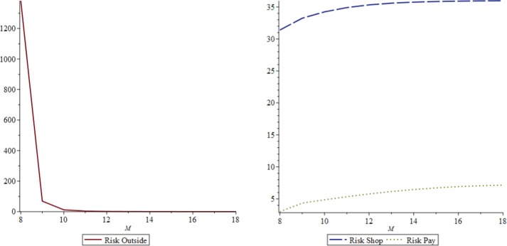
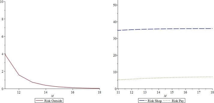
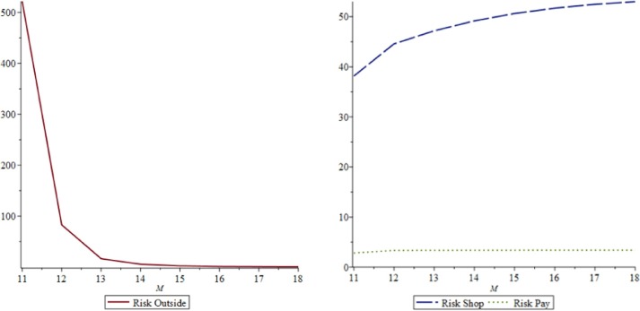
By substituting the store’s best response, $c(M)$ for the M-model and $c(M)\text{and}N(M)$ for the NM-model, the risk measures $E\left[L(L-1)\right]$ as a function of M are obtained for each queue. See Fig. 12a, Fig. 12b for the M-model and Fig. 13 for the NM-model.

Fig. 12a.

Effect of M on $E\left[L(L-1)\right]$ in the M-model.

Fig. 12b.

Effect of $M⩾11$ on $E\left[L(L-1)\right]$ in the M-model.

Fig. 13.

Effect of M on $E\left[L(L-1)\right]$ in the NM-model.

As depicted in Fig. 12a, Fig. 12b, Fig. 13, the risk of being infected for customers waiting outside is much greater under the NM-model. The risk for customers in the shopping phase is less under the M-model than under the NM-model, and the risk for customers in the payment phase is less under the NM-model than under the M-model. Moreover, payer risk under the NM-model is relatively stable since the number of payers who can occupy the space is limited. Under the M-model, payer risk increases with M.

The store’s equilibrium strategy also depends on the values of the weights assigned by the authority to each measure of risk. Set ${\mathit{\alpha }}_1=1,{\mathit{\beta }}_2=100,{\mathit{\beta }}_3=100$. These weights reflect the position that waiting in line outside where social distance can be maintained presents a much lower risk than waiting inside the store. For this example, the equilibrium strategy is $M^{\ast }=11,c^{\ast }=3$ under the M-model and $M^{\ast }=16,c^{\ast }=3,N^{\ast }=2,K^{\ast }=11$ under the NM-model. We also consider a scenario in which the risk of being infected while waiting in line in the payment phase is greater than the risk of being infected in the shopping phase: ${\mathit{\alpha }}_1=1,{\mathit{\beta }}_2=100,{\mathit{\beta }}_3=500.$ In that case, the store’s equilibrium strategy is $M^{\ast }=9,c^{\ast }=3$ under the M-model and $M^{\ast }=14,c^{\ast }=3,N^{\ast }=1,K^{\ast }=10$ under the NM-model.

It follows from these results that, when the risk of being infected in the payment phase is greater than the risk of being infected in the shopping phase, the authority reduces the number of customers allowed in the store by 2: from 11 to 9 under the M-model and from 16 to 14 under the NM-model. Because of this reduction in the number of customers allowed in, the store in the NM-model reduces the maximum number of customers in the shopping phase ($K^{\ast }$) and the maximum number of customers in the payment phase ($N^{\ast }$).

6. Conclusion

In this paper, we construct and analyze two special nonclassical multi-server queueing models to control queueing problems generated by social distancing constraints associated with the COVID-19 pandemic such as “Maximum shoppers at store” and “maximum number of customers in checkout area.” In both models, a capacity constraint is imposed that limits the number of customers allowed inside the store at one time. The governing authority that imposes the limit acts as a Stackelberg leader in choosing how many customers will be allowed. Then, store management chooses the number of cashiers to employ to reduce its costs in terms of cashier salaries and the cost of dissatisfaction from customers waiting in line. In the second model, store management can also choose a maximum number of customers who can occupy a separate payment area in a queue formed in front of the cashiers. For each model, we derive and analyze the equilibrium strategies in terms of the store’s customer capacity and the number of cashiers. Our findings are useful and applicable for both government authorities imposing restrictions and the businesses subject to the restrictions in their efforts to ensure the safety of customers and employees while reducing associated costs.

References

- Alban, A., Chick, S.E., Dongelmans, D.A., van der Sluijs, A.F., Wiersinga, W.J., Vlaar, A.P., Sent, D., 2020. ICU capacity management during the COVID-19 pandemic using a stochastic process simulation. [DOI] [PMC free article] [PubMed]
- Avrachenkov K., Nain P., Yechiali U. A retrial system with two input streams and two orbit queues. Queueing Syst. 2014;77(1):1–31. [Google Scholar]
- Barr G.D. The Covid-19 Crisis and the need for suitable face masks for the general population. Chinese J. Med. Res. 2020;3:28–31. [Google Scholar]
- BBC News, 2020. https://www.bbc.com/news/uk-england-52051322. March 27.
- CNN, 2020. https://edition.cnn.com/2020/05/18/us/coronavirus-time-risk/index.html. May 18.
- Government of the United Kingdom, 2020. Keeping Workers and Customers Safe during COVID-19 in Restaurants, Pubs, Bars, and Takeaway Services. https://assets.publishing.service.gov.uk/media/5eb96e8e86650c278b077616/working-safely-during-covid-19-restaurants-pubs-bars-takeaway-090720i.pdf.
- Gupta, M., Abdelsalam, M., Mittal, S., 2020. Enabling and enforcing social distancing measures using smart city and its infrastructures: a COVID-19 Use case. arXiv preprint arXiv:2004.09246.
- Hanukov G., Yechiali U. Explicit solutions for continuous-time QBD processes by using relations between matrix geometric analysis and the probability generating functions method. Prob. Eng. Inform. Sci. 2020:1–16. [Google Scholar]
- Harchol-Balter M. Cambridge University Press; 2013. Performance Modeling and Design of Computer Systems: Queueing Theory in Action. [Google Scholar]
- Israeli i24News, 2020. https://www.i24news.tv/en/news/israel/1588829440-israel-malls-fitness-centers-set-to-reopen-thursday-as-virus-cases-dip. (May 07, 2020).
- Kaplan E.H. OM Forum—COVID-19 scratch models to support local decisions. Manuf. Service Operat. Manage. 2020;22(4):645–655. [Google Scholar]
- Long, D.Z., Wang, R., Zhang, Z., 2020. Pooling and Balking: Decisions on COVID-19 Testing. Available at SSRN 3628484.
- Neuts M.F. Matrix-geometric solutions in stochastic models: an algorithmic approach. The Johns Hopkins University Press, Baltimore, MD. 1981 [Google Scholar]
- Perel N., Yechiali U. The Israeli queue with retrials. Queueing Syst. 2014;78(1):31–56. [Google Scholar]
- Perlman Yael, Elalouf Amir, Yechiali Uri. Dynamic allocation of stochastically-arriving flexible resources to random streams of objects with application to kidney cross-transplantation. Europ. J. Operat. Res. 2018 doi: 10.1016/j.ejor.2017.07.068. [DOI] [Google Scholar]
- Perlman Y., Yechiali U. On tandem stochastic networks with time-deteriorating product quality. Int. J. Prod. Res. 2020;58(13):3956–3964. [Google Scholar]
- Winkler M., Perlman Y., Westreich S. Reporting near-miss safety events: Impacts and decision-making analysis. Safety Sci. 2019;117:365–374. [Google Scholar]