Effect of removing outliers on statistical inference: implications to interpretation of experimental data in medical research

Abstract

Background

Data editing with elimination of “outliers” is commonly performed in the biomedical sciences. The effects of this type of data editing could influence study results, and with the vast and expanding amount of research in medicine, these effects would be magnified.

Methods and Results

We first performed an anonymous survey of medical school faculty at institutions across the United States and found that indeed some form of outlier exclusion was performed by a large percentage of the respondents to the survey. We next performed Monte Carlo simulations of excluding high and low values from samplings from the same normal distribution. We found that removal of one pair of “outliers”, specifically removal of the high and low values of the two samplings, respectively, had measurable effects on the type I error as the sample size was increased into the thousands. We developed an adjustment to the t score that accounts for the anticipated alteration of the type I error (t_adj=t_obs-2(log(n)^0.5/n^0.5)), and propose that this be used when outliers are eliminated prior to parametric analysis.

Conclusion

Data editing with elimination of outliers that includes removal of high and low values from two samples, respectively, can have significant effects on the occurrence of type 1 error. This type of data editing could have profound effects in high volume research fields, particularly in medicine, and we recommend an adjustment to the t score be used to reduce the potential for error.

Introduction

There has been an ongoing debate for more than two decades as to the reproducibility and reliability of published medical research.^1,2 Ioannidis³ modeled the positive predictive value (PPV) of a research finding as a function of bias, defined as “the combination of various design, data, analysis, and presentation factors that tend to produce research findings when they should not be produced,” demonstrating that an increase in bias results in a decrease in PPV for commonly-occurring values of statistical power and thresholds for statistical significance. Consequently, the interpretation of published research findings as “true” presupposes a low level of bias in research methodology. With some notable exceptions of scientists presenting false results in an egregious manner, it is generally assumed that scientists by and large present their data in an ethical and conservative manner.⁴

That said, it is also clear that many scientific laboratories exclude some data from publication for a variety of reasons.⁵ In some cases, it is because one or more data points are really “different” from the rest of the experimental results.⁶ In other cases, it is because these outliers either affect regression analysis substantially or cause the t-test to yield a non-significant value with significance defined as an alpha error < 5%.^7–9 In addition, there is significant variability in how an outlier is defined; some use the two or three sigma rule, while others use the boxplot and interquartile range method of Tukey, or even simply identify outlier values graphically.^10–12 Regardless of the reason or method of identification, this type of data editing has the potential to create type 1 error, i.e. a statistically significant difference discovered when in reality it does not exist.

The creation of type 1 error can have a dramatic impact, particularly in the growing and expanding fields of medical research. From the year 2000 to 2010, it is estimated that nearly 80,000 journal articles were published in the field of cardiovascular disease alone.¹³ Therefore, even if a small proportion of type 1 error is introduced, the effects would be enormous. In addition, research with significant findings, including that with type 1 error, is developed and expanded upon, potentially multiplying the problem.

To better understand the extent to which outlier exclusion occurs, and to illustrate how it may increase bias, we performed the following survey of US medical school faculty and Monte Carlo simulations using the open source program R along with published packages.

Methods

Survey of Medical School Faculties

We performed a survey of all US allopathic medical schools. This survey was deemed exempt by the Marshall institutional review board. We contacted each dean of an allopathic medical school with a personal email requesting that a link to our survey, created with SurveyMonkey™ (SurveyMonkey, Inc., San Mateo, CA, USA), be distributed among medical faculty at the school. A copy of the survey is shown in appendix A. The survey was developed by experts in biomedical research and biostatistics and was felt to have acceptable face validity. Internal consistency was high as measured by Cronbach’s alpha for two similar questions relating to the management of outlier values (alpha = 0.71).

We received a response from most of the medical school deans agreeing to our request. Five of the 40 schools that responded had policies against distribution of such surveys and respectfully declined. As the survey was anonymous, we cannot assess our response rate to any degree nor did we try to track who responded from which institution. With the large mailing described above, we received 1152 total responses from medical school faculty members.

We reported the proportionate responses to our survey questions (Appendix) and provided a summary of key responses in the results section. To evaluate characteristics of our survey respondents associated with excluding outliers, we used the survey question that asked about the exclusion of outliers when performing a Student’s t test and dichotomized the responses into ‘exclude outliers’ versus all other responses. We then performed simple logistic regression examining the association of’excluding outliers’ with survey respondent self-reported characteristics. Stata 15.0 (College Station, TX) was used for analysis of survey results.

Monte Carlo Simulations

The open source program R was used for all simulations in this study.¹⁴ To model the effect of outlier exclusion on computed p-values of experiments for which the null hypothesis held, we first drew two data sets from the same normal distribution (mean of 1, SD of 1 unless otherwise stated) with the same sample size in each set 10,000 times. In the control case, we did not modify these sets and performed tests of significance (either t-test or Mann-Whitney U test). In the experimental case, we removed one or more of the highest values from one of the two sets and one or more of the lowest values from the other set prior to performing these statistical tests. Data are presented graphically. The basic R code used for these simulations is attached as appendix II.

Results

Survey

A survey instrument was developed and furnished to the members of the Council of Deans with the request to share the survey link with their faculty. The majority of these medical school deans agreed to distribute this survey link, and we obtained 1152 anonymous responses. Among the 1152 medical school faculty respondents, 800 (69.4%) completed all questions on demographics, academic background, and statistics regarding outliers and will serve as the focus for analysis of our survey results.

Most survey respondents were between the ages of 35 to 64 (75.2%) and 515 (N=64.4%) were male. Academic rank was fairly evenly distributed with 29.7% assistant professor, 25.4% associate professor, and 42.4% professor (remainder either not reported (0.6%) or instructor (1.9%)). Faculty reported a broad range of time spent in research: 1-5 years (25.0%) to >20 years (38.0%). There were 351 (43.7%) with an MD or DO degree, 361 (45.0%) with a PhD degree, and 44 (5.9%) with a combined MD or DO/PhD degree. The majority of faculty reported formal training in statistics (56.6%) and most reported that they either ‘perform their own statistics’ (29.4%) or ‘perform their own statistics and use someone else’ to help them (33.5%), while roughly a third of faculty (32.4%) reported that they have ‘someone else perform statistics for their research studies.’ Finally, 74.6% of faculty reported that a statistician was available to assist with statistics.

We asked faculty if they generally explored the distribution of a continuous variable and 74.0% responded ‘yes.’ We asked faculty how they handled outlier values when describing a continuous variable. Fewer than half of faculty (46.9%) reported that they ‘use all data in the descriptive analysis, including outliers’, while 20.1% of faculty reported that they exclude outlier values (11.2% reported running a formal outlier test). Faculty responded similarly to the question regarding analysis of a continuous variable using the Student’s t test with 19.0% excluding outlier values from the bivariate analysis.

We examined the association of excluding outliers in statistical analysis with self-reported characteristics of those surveyed (Figure 1). We found that those with a PhD degree were nearly twice as likely (OR 1.9, 95% CI 1.3 – 3.0) to exclude outliers compared to those with an MD or DO degree. We also found that those who perform their own statistics (with or without a statistician) were more likely (OR 1.9, 95% CI 1.3 – 2.8) to exclude outliers compared to those who do not perform their own statistics. We found no association to ‘exclude outliers’ with academic rank, years of research experience, formal training in statistics, and having the availability of a statistician.

Figure 1.

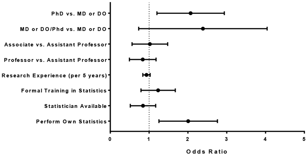
Odds of Excluding Outlier Values in Bivariate Analysis using the Student’s T Test by Self-Reported Characteristics of Survey Respondents. Error bars represent the 95% confidence interval.

Outlier Data Editing Simulation

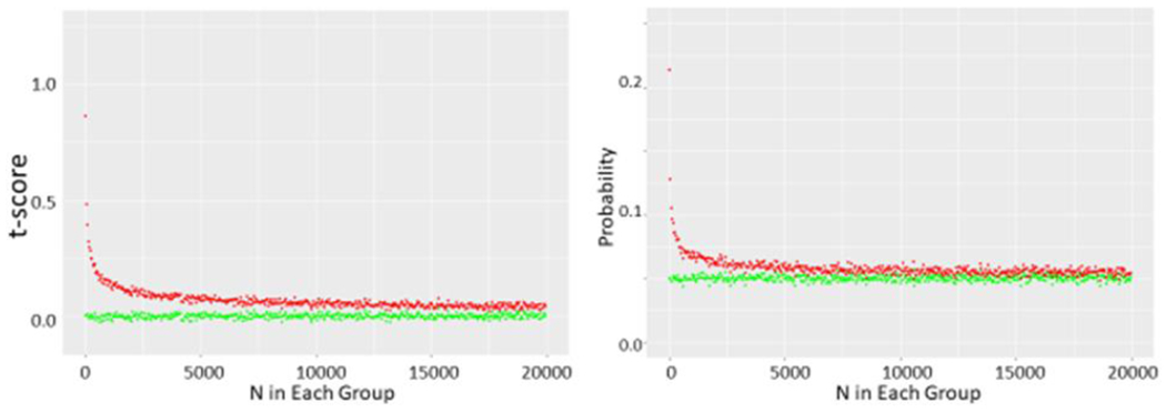
Using Monte Carlo simulations, we found that simply drawing the different data sets from the normal distribution resulted in t-tests yielding p<0.05 just about 5% of the time as expected as N was incremented from N=10 through N= 10,000 in each data set. However, if we removed the highest data point from one set and the lowest value from the other, a significant shift in the t distribution is seen (Figure 2a) with t scores corresponding to a p<0.05 value in just over 20% of simulations with N=10 in each group (Figure 2b). As we increased N further, we saw the chance of a t-test indicating a p<0.05 decrease further, but it was still markedly greater than 5% of cases as N was increased through several thousand (Figure 2c). As expected, this did not appear to be related to the SD (Figure 3, data shown for N=10 in each group). Increasing the number of data points removed increased this chance as expected while removing 5 data points from each N=10 data set nearly guaranteed statistically significant differences (Figure 3c). While the non- parametric Wilcoxon test was less susceptible to the outlier removal effect, elevated chances of detecting “significant” differences (p<0.05 or p<0.01) were observed through N=50 in each set (Figure 4).

Figure 2.

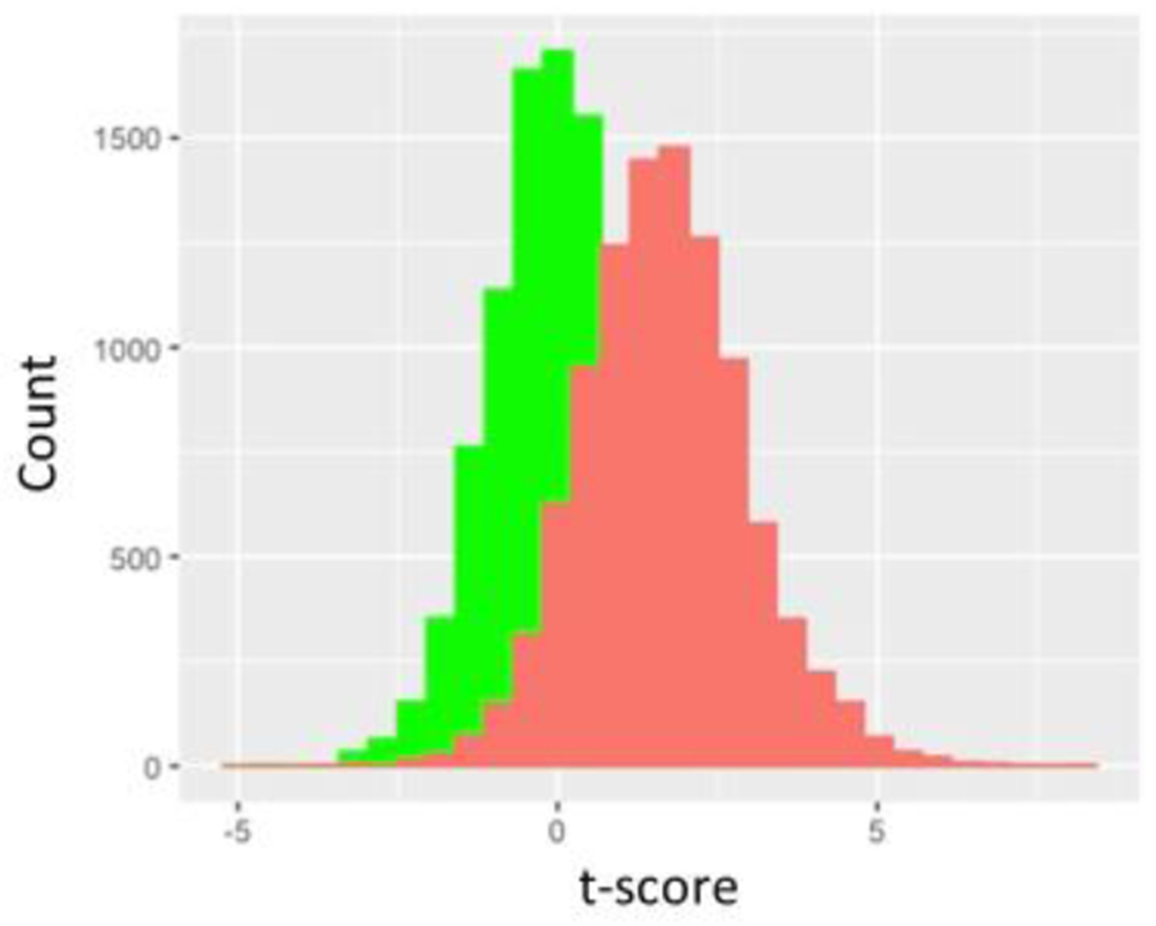
a shows green histogram for 10,000 t-scores determined by drawing two N=10 samples from a normal distribution with mean of 1 and SD of 1. Red histogram is also 10,000 t-scores determined by these same pairs of N=10 samples from same underlying distribution except highest value of one sampling and lowest value of the other sampling are systematically eliminated.

b shows t scores and corresponding p values obtained from running 10,000 t-tests on N samples drawn from this same normal distribution and corresponding p values where N ranges from 5 to 25. Green circles represent unmodified pairs of samples whereas red circles represent sets where top value of one and bottom value of other sample are dropped.

c shows data obtained as N ranges from 10 to 20,000 in each set.

Figure 3.

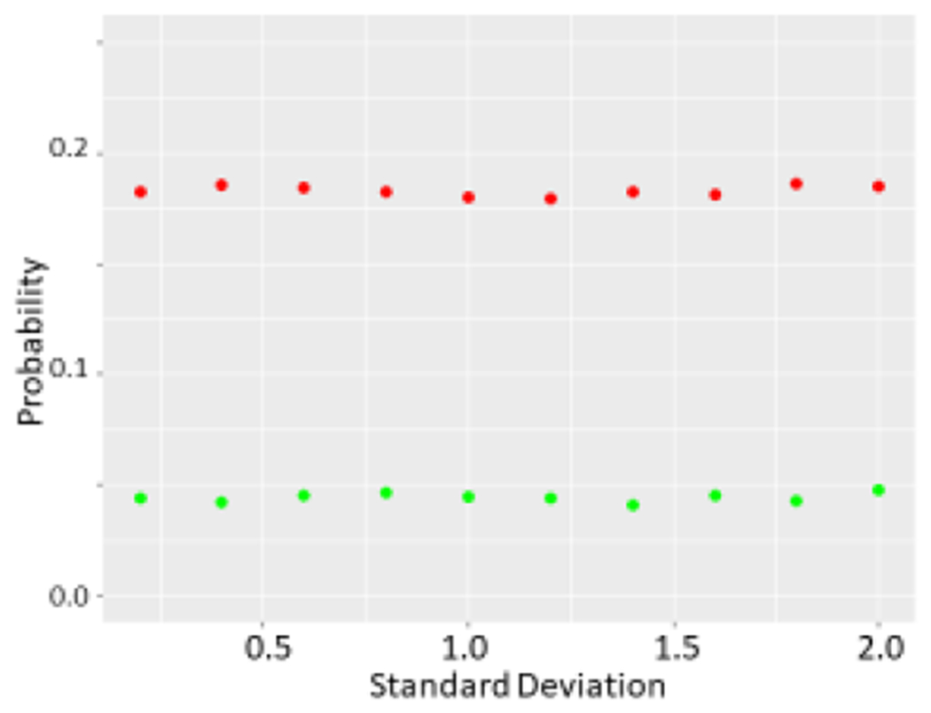
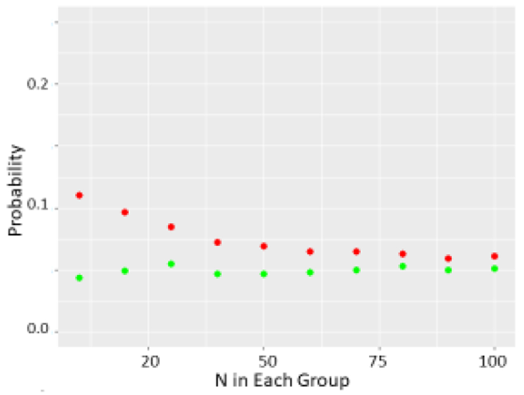
a The effect of varying SD on probability of a p<0.05 difference determined by the t-test. Again green refers to unmodified sets whereas red refers to sets where top value of one and bottom value of other are dropped. N=10 was used for unmodified sets.

b Wilcoxon test performed on two sets as described previously as N was allowed to range from 10 to 100.

c Probability of obtaining a p<0.05 value with initial N=10 in each group (green) as the number of pairs of top and bottom values which are dropped (red) is increased from 1 to 5.

Figure 4.

Fit of formula 2*(log(n)^.5/(n^0.5) (purple small dots) to mean t-values determined with 10,000 simulations performed as N was increased from 10-20,000 with no modification (green) or single top and bottom values from data set pairs dropped (red).

We used the following formula to estimate the expected max-min of drawing N values from a normal distribution¹⁵ as

$${\text{E}\left(\text{max}\right)-\text{E}\left(\text{min}\right)=2*\text{SD}*(2*\text{log}(\text{n}\left)\right)}^{0.5}$$ (1)

This yielded the correction that “dropping” a pair of outliers from sampling n values in each set would create a variation in t score given by

$${\text{t}}_{\text{obs}}-{\text{t}}_{\text{corr}}{=2*\left(\text{log}\right(\text{n}\left)\right)}^{\text{0}.5}/{\text{n}}^{0.5}\text{)}$$ (2)

With this formula, we estimated with fair accuracy the observed deviation in t score from this type of data editing (Figure 4). We further suggest that a reasonable estimate for dropping p pairs of such outliers is to simply multiple the right hand of (2) by p.

Discussion

We believe our study is interesting in several ways. First and foremost, as shown by the survey results, some degree of data editing is commonly performed by biomedical researchers. However, the implications of such data editing may not be well appreciated.⁵ Frankly, the authors of this paper were somewhat surprised by the degree to which the effect of dropping an outlier pair persisted as n increased. While this perhaps should not have been surprising given that the term log(n)^0.5/n^0.5 approaches zero rather slowly as n increases, we would not have predicted that a measurable effect of removing a single outlier pair existed when n was in the thousands. This is particularly surprising given the fact that the “outlier pair” in our simulations consisted of high and low values, a reasonable yet conservative approach. An even more dramatic effect would be expected when using actual outlier pairs that would be farther from the central tendency of the data than high and low values. Given the vast and ever expanding number of publications in medical research, use of this type of data editing could introduce type 1 error and could have grave effects on study outcomes.

It is perhaps notable that faculty who performed their own statistical analysis (i.e. without the help of a statistician) were more likely to perform outlier removal (Figure 1). While the extent of the effect of outlier removal is likely known, or at least readily accessible to the statistical community, the results of the simulations we performed are likely to be highly illustrative to medical researchers who may have less statistical expertise. While some degree of data editing is probably unavoidable in biomedical science, we further suggest that some correction to the Student t-test be performed for such outlier elimination as has become commonplace with post- hoc t-tests involving multiple comparisons.

Appendix I: Survey Instrument/Results

Selected questions and responses to survey in 800 participants with complete data on demographics and initial statistics question.

What is your age?

Answer Choices	N	Percent
25 to 34	44	5.5
35 to 44	190	23.8
45 to 54	202	25.2
55 to 64	210	26.2
65 to 74	126	15.8
75 to older	28	3.5

What is your gender?

Answer Choices	N	Percent
Female	285	35.6
Male	515	64.4

What is your current academic position?

Answer Choices	N	Percent
Instructor	15	1.9
Assistant Professor	238	29.7
Associate Professor	203	25.4
Professor	339	42.4
Not reported	5	0.6

What degrees do you hold? (Categories are not mutually exclusive)

Answer Choices	N	Percent
MS	109	13.6
MPH	57	7.1
MD	397	49.6
PhD	406	50.8
DrPh	5	0.6
Other	64	8.0

How long have you been involved in research?

Answer Choices	N	Percent
1-5 years	200	25.0
6-10 years	83	10.4
11-15 years	84	10.5
15-20 years	126	15.7
More than 20 years	304	38.0
Not reported	3	0.4

Who performs the statistics for your research studies?

Answer Choices	N	Percent
I perform my own statistics for my research studies	235	29.4
I have someone else perform statistics for my research studies	259	32.4
I perform my own statistics and use someone else to perform statistics for my research studies	268	33.5
Other	38	4.7

Have you had formal training in research statistics?

Answer Choices	N	Percent
Yes	453	56.6
No	347	43.4

Do you have a statistician to assist you with statistics in your research studies?

Answer Choices	N	Percent
Yes	596	74.6
No	203	25.4
No response	1	0.0

Do you generally explore the distribution (normal vs. non-normal) of continuous variables used in your research to make sure the appropriate statistics (parametric vs. non-parametric) are used?

Answer Choices	N	Percent
Yes	592	74.0
No	140	17.5
Other	68	8.5

Which of the following do you use to assess the distribution of a continuous variable?

Answer Choices	N	Percent
Graphs, such as histograms, stem and leaf plots, normal plots, etc.	208	26.0
Statistical tests, such as the Shapiro-Wilk or Shapiro-Francia	88	11.0
Both graphs and statistical tests	439	54.9
Other	65	8.1

When describing a continuous variable that is normally distributed with the mean and the standard deviation, how do you handle outliers?

Answer Choices	N	Percent
I use all data in the descriptive analysis, including outliers	375	46.9
I remove outliers from the descriptive analysis	71	8.9
I use the median and interquartile range instead to describe the variable	107	13.4
I always run an outlier test (Grubb’s test or similar) on my data and remove points that are marked as outliers and then perform the descriptive analysis	90	11.2
Other	144	18.0
No response	13	1.6

When analyzing a continuous variable that is normally distributed with the Student’s t test, how do you handle outlier values for that continuous variable?

Answer Choices	N	Percent
I use all data in the bivariate analysis, including outliers	332	41.5
I exclude outliers from the bivariate analysis	62	7.8
I use a nonparametric method for bivariate analysis, such as the Mann-Whitney test	139	17.4
I always run an outlier test (Grubb’s test or similar) on my data and remove points that are marked as outliers and then perform the bivariate analysis	90	11.2
Other	144	18.0
No response	33	4.1

Appendix II: R Code

# load libraries

library(ggplot2)

library(dplyr)

library(tidyverse)

#set up matrices

A=NULL

Experimental=NULL

Control=NULL

BB=NULL

CC=NULL

DD=NULL

EE=NULL

CT=NULL

ET=NULL

ME=NULL

MM=NULL

# number of measurements (k below) or could vary SD if you wanted

# r is number of “outliers” removed

# LL is number of loops for varying k or SD

# must adjust N at end of program as well for graphs

set.seed(6)

LL=20

for(j in 1:LL){

# loop through simulation 10,000 times, much less and variability is

# obfuscating

for(i in 1:10000){

k=j+4 #set up to vary k= 5 through 25 in this set

r =1 #remove 1 from each set

#draw k values from a normal distribution with mean=1 and SD = 1

x1a=rnorm(k,1,1)

x2a=rnorm(k,1,1)

#throw out lowest value from first set and highest value from second set

x1b=x1a[rank(x1a, ties.method = “first”) > r]

x2b=x2a[rank(x2a, ties.method = “first”) <= k-r]

# could also set up with wilcoxon

# results more “interesting with #t.test (of course)

# B=wilcox.test(x1a,x2a,”greater”)

# C=wilcox.test(x1b,x2b,”greater”)

B=t.test(x1a,x2a, “greater”)

C=t.test(x1b,x2b,”greater”)

#capturing p values

Control[i]=B[3]$p.value

Experimental[i]=C[3]$p.value

# capturing t-score

m=B[1]

m=as.data.frame(m)

n=C [1]

n=as.data.frame(n)

CT[i]=m [1,1]

ET[i]=n[1,1]

}

# after you loop 10,000 times we count

# p values

BB[j]=length(subset(Control,Control<0.05))/10000

DD[j]=length(subset(Experimental,Experimental<0.05))/10000

#t-scores

MM[j]=mean(CT)

ME[j]=mean(ET)

}

#set up graphs

#make everything into dataframes

K=seq(1:LL)

BB=as.data.frame(BB)

DD=as.data.frame(DD)

N=K+4

#plot data for p<0.05

#controls are green, sets with data removed are red

p=ggplot(BB)+geom_point(aes(x=N,y=BB),colour=“green”,size=1)+geom_point(aes(x=N,y=DD),colour=“red”,size=1)+ylab(“Probability”)+xlab(“N in Each Group”)+coord_cartesian(ylim=c(0,0.25))

plot(p)

# set up correction to t graph

xxx=2*log(N)^.5

yyy=N^0.5

zz=xxx/yyy

# plot t score +/− correction

q=ggplot(BB)+geom_point(aes(x=N,y=MM),colour=“green”,size=3)+geom_point(ae s(x=N,y=ME),colour=“red”,size=3)+geom_point(aes(x=N,y=zz),col=“purple”)+yl ab(“t-score”)+xlab(“N in Each Group”)+coord_cartesian(ylim=c(−0.1,1.25))

plot(q)

#

q=ggplot(BB)+geom_point(aes(x=N,y=MM),colour=“green”,size=1)+geom_point(ae s(x=N,y=ME),colour=“red”,size=1)+ylab(“t-score”)+xlab(“N in Each Group”)+coord_cartesian(ylim=c(−0.1,1.25))

# plot(q)

References

- 1.Altman DG. The scandal of poor medical research. BMJ. 1994;308(6924):283–4. 10.1136/bmj.308.6924.283 [DOI] [PMC free article] [PubMed] [Google Scholar]
- 2.Hanin L Why statistical inference from clinical trials is likely to generate false and irreproducible results. BMC Med Res Methodol. 2017;17(1):127 10.1186/s12874-017-0399-0 [DOI] [PMC free article] [PubMed] [Google Scholar]
- 3.Ioannidis JP. Why most published research findings are false. PLoS Med. 2005;2(8):e124 10.1371/journal.pmed.0020124 [DOI] [PMC free article] [PubMed] [Google Scholar]
- 4.Wade N, Broad WJ. Betrayers of the truth. First ed: New York: Simon and Schuster; 1983. [Google Scholar]
- 5.Altman N, Krzywinski M. Analyzing outliers: influential or nuisance? Nat Methods. 2016;13(4):281–2. 10.1038/nmeth.3812 [DOI] [PubMed] [Google Scholar]
- 6.Tabatabaee H, Ghahramani F, Choobineh A, Arvinfar M. Investigation of outliers of evaluation scores among school of health instructors using outlier - determination indices. J Adv Med Educ Prof. 2016;4(1):21–5. [PMC free article] [PubMed] [Google Scholar]
- 7.Beath KJ. A finite mixture method for outlier detection and robustness in meta-analysis. Res Synth Methods. 2014;5(4):285–93. 10.1002/jrsm.1114 [DOI] [PubMed] [Google Scholar]
- 8.Fomenko I, Durst M, Balaban D. Robust regression for high throughput drug screening. Comput Methods Programs Biomed. 2006;82(1):31–7. 10.1016/j.cmpb.2006.01.008 [DOI] [PubMed] [Google Scholar]
- 9.Jamrozik J, Stranden I, Schaeffer LR. Random regression test-day models with residuals following a Student’s-t distribution. J Dairy Sci. 2004;87(3):699–705. 10.3168/jds.s0022-0302(04)73213-0 [DOI] [PubMed] [Google Scholar]
- 10.Ben-Gal I Outlier Detection [w:] Data Mining and Knowledge Discovery Handbook: A Complete Guide for Practitioners and Researchers, red. Maimon O, Rokach L. Kluwer Academic Publishers, Boston; 2005. 10.1007/978-0-387-09823-4_7 [DOI] [Google Scholar]
- 11.Pukelsheim F The three sigma rule. The American Statistician. 1994;48(2):88–91. 10.2307/2684253 [DOI] [Google Scholar]
- 12.Tukey JW. Exploratory data analysis: Reading, Mass.; 1977. [Google Scholar]
- 13.Biglu M-H, Ghavami M, Biglu S. Cardiovascular diseases in the mirror of science. Journal of Cardiovascular and Thoracic Research. 2016;8(4):158–63. 10.15171/jcvtr.2016.32 [DOI] [PMC free article] [PubMed] [Google Scholar]
- 14.Quick JM. Statistical analysis with R beginners guide: take control of your data and produced superior statistical analysis with R. Birmingham: Packt Publ; 2010. [Google Scholar]
- 15.Santner TJ, Duffy DE. The statistical analysis of discrete data. Springer texts in statistics; www.springer.com: Springer; 1991:367 10.1007/978-1-4612-1017-7 [DOI] [Google Scholar]