Figure 15.

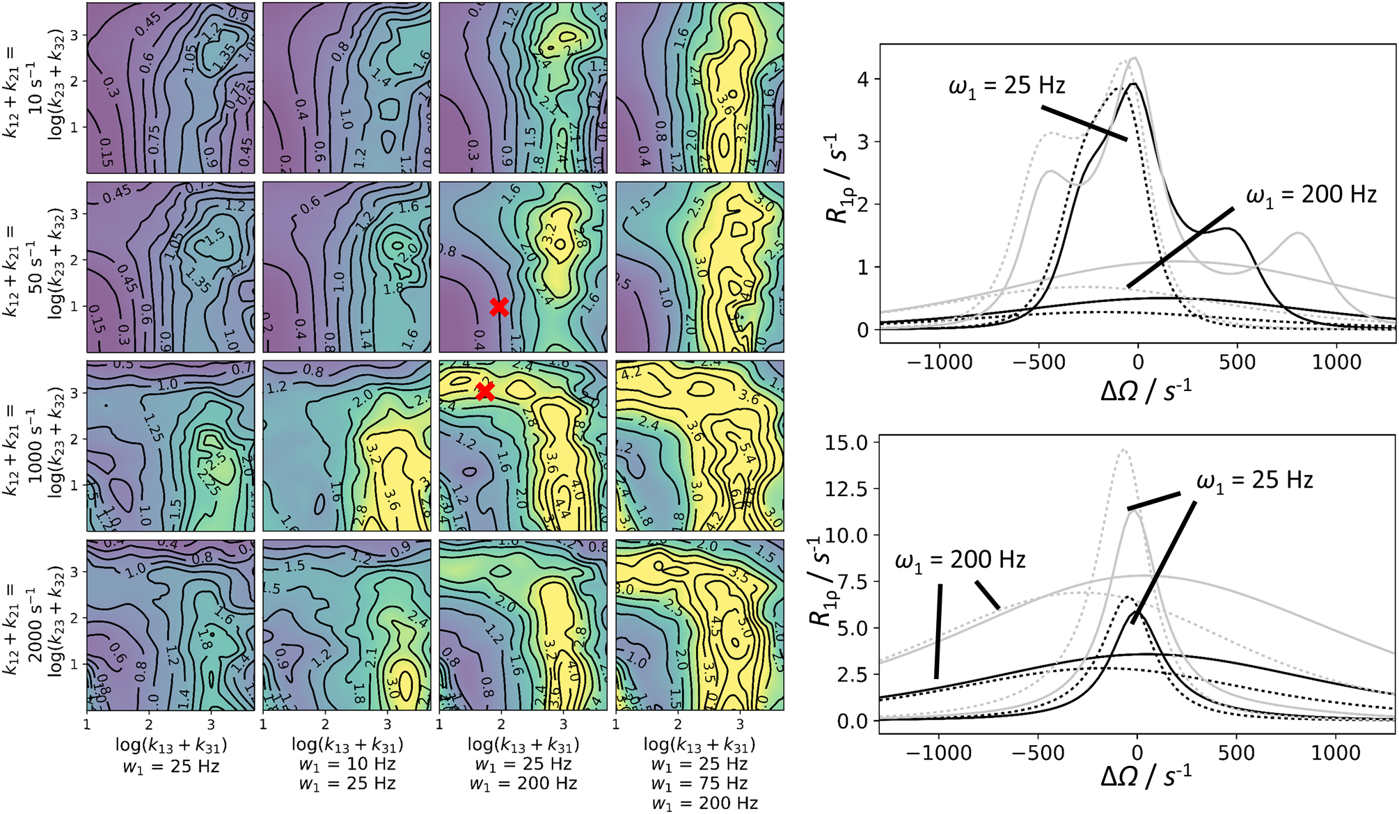
Distinguishability of the 3-state linear and triangular kinetic scheme from the two-state model in R_1ρ experiments. Left panel: General conditions for distinguishability. Each subpanel has been created from 90 data points; each corresponds to the median of 20 separately calculated RMS values. For each RMS value, five sets of spins with randomly generated chemical shifts Δω_AB (200–800 s⁻¹ at 11.7 T) and Δω_AC (±200–800 s⁻¹) were included. In addition, two B₀ fields (11.7 T, 18.7 T) and various combinations of one to three ω₁ fields (see figure) were used. This yielded 10 to 30 numerically generated R_1ρ curves for three sites. These curves were globally fit to a two-site model (ΔΩ range: −1300 to 1300 s⁻¹). The RMS for each of the synthetic and fitted curve combinations was calculated. The results are shown in the contour plot. The points from which the sample fits in the right panels were generated are marked. Multiple parameters are shown in the plot, other parameters are: p_B = 0.05; p_C = 0.02. To aid in convergence, some variables were constrained between upper and lower bounds during fitting: p_B between 0.005 and 0.23; k₁₂ + k₂₁ between 5 s⁻¹ and 7000 s⁻¹; Δω_AB between 100 s⁻¹ and 1200 s⁻¹. Right panel: Example curves corresponding to various kinetic situations marked in the right panel (top: k₁₂ + k₂₁ = 50 s⁻¹; k₁₃ + k₃₁ = 100 s⁻¹; k₂₃ + k₃₂ = 10 s⁻¹; ω₁/(2π) = 25 and 200 Hz; bottom: k₁₂ + k₂₁ = 1000 s⁻¹; k₁₃ + k₃₁ = 50 s⁻¹; k₂₃ + k₃₂= 1000 s⁻¹; ω₁/(2π) = 25 and 200 Hz). Numerical three-state solutions (solid lines) are shown alongside the best two-state fits (dotted lines). The fits result from global fits of 20 curves: five spins (in plot only shown: Δω_AB = 536 s⁻¹; Δω_AC = −312 s⁻¹); B₀ = 11.7 T, black; B₀ = 18.7 T, grey; ω₁/(2π) = 50 Hz and 200 Hz, as indicated in the figure. The RMS deviation for the given examples are 0.74 s⁻¹ (top) and 3.48 s⁻¹ (bottom).