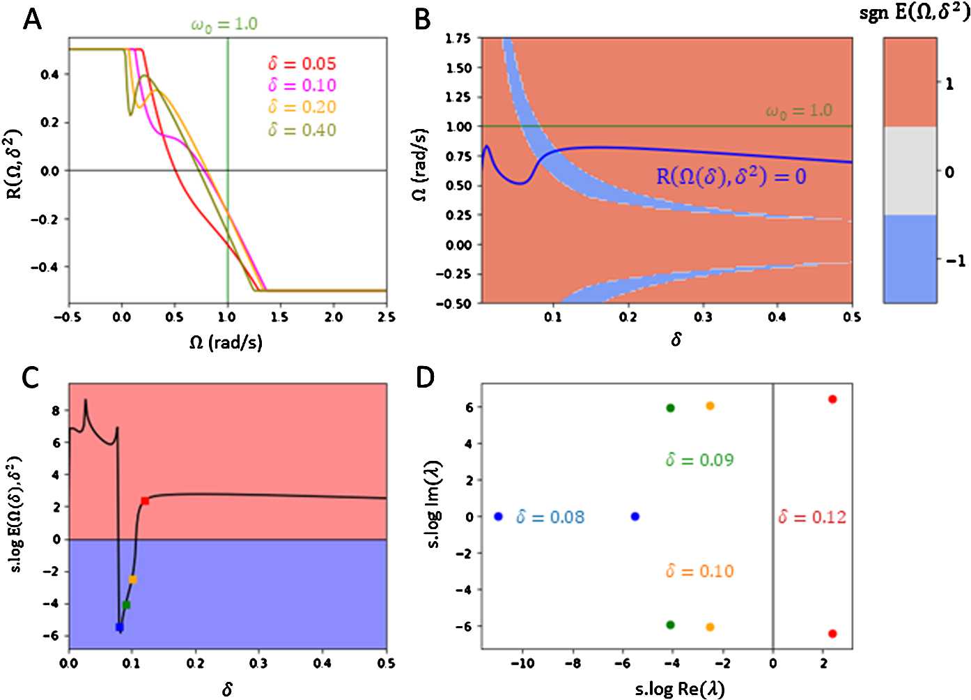
Figure 3.

Theoretical stability plots for large N-dim oscillator system. A. Plots of error function $\mathcal{R}(\Omega ,{\delta }^2)$ with varying fixed $\delta >0$ over $\Omega \in [{\omega }_0-g,{\omega }_0+g]$. The function is truncated between interval $[-0.5,0.5]$ for visibility. There is a unique root $\mathcal{R}(\Omega ,{\delta }^2)=0$ for each fixed $\delta >0$. B. Colour map of $sgnE(\Omega ,{\delta }^2)$ over states $(\Omega ,{\delta }^2)\in [{\omega }_0-g,{\omega }_0+g]\times (0,{0.5}^2)$, along with the implicit solution curve (purple) $\Omega =\Omega (\delta )$ parametrizing level set $\mathcal{R}(\Omega ,{\delta }^2)=0$. Stable regions correspond to $sgnE(\Omega ,{\delta }^2)=-1$ (blue) and unstable regions correspond to $sgnE(\Omega ,{\delta }^2)=1$ (red). The network synchronizes near a state $(\Omega (\delta ),{\delta }^2)$ overlapping the stable region. C. Plot of stability term $\text{s.}logE(\Omega ,{\delta }^2)$ along the solution curve $\Omega =\Omega (\delta )$ over $\delta \in (0,0.5)$. There is a small interval $\delta \in (0.08,0.1)$ for which $(\Omega (\delta ),{\delta }^2)$ is in the stable region (blue). Other states are in the unstable region (red). D. Complex plot of non-zero eigenvalues of $P(\lambda \mid \Omega ,{\delta }^2)+Q(\lambda \mid \Omega ,{\delta }^2)$ on solution states $(\Omega ({\delta }^2),{\delta }^2)$ across varying $\delta >0$, scaled by s.log for visibility. The eigenvalues in plot D were computed at respective states $(\Omega ,{\delta }^2)$ in plot C indicated by the same colour. Power terms for polynomial $Q(\lambda \mid \Omega ,{\delta }^2)$ were computed up to degree $M=3$. The parameters used for all plots are ${\alpha }_{\tau }=1.0$, $g=1.5$, ${\omega }_0=1.0$, $\kappa =80$, and ${\tau }^0=0.1\text{s}$