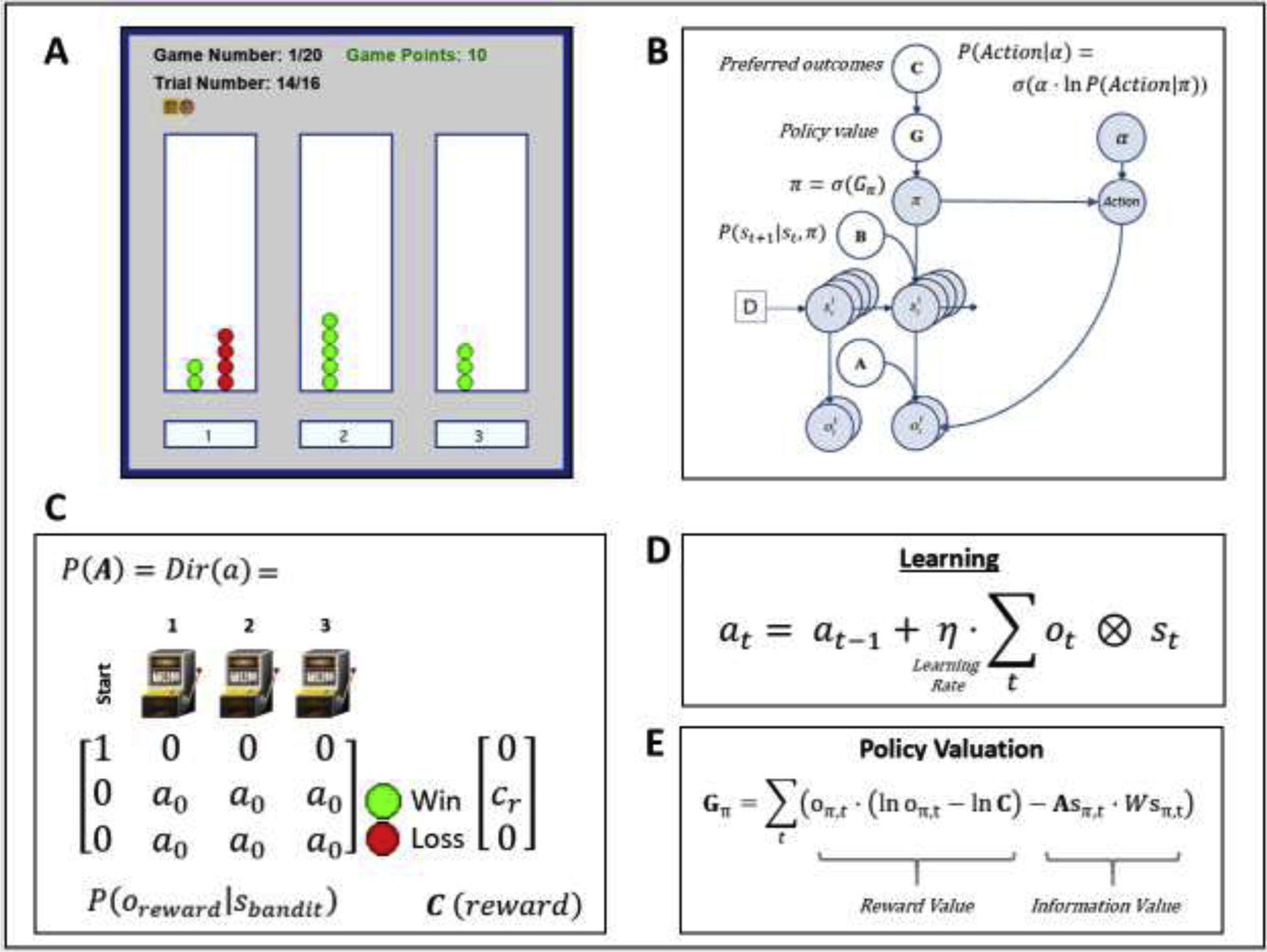
Figure 1.

(A) Illustration of the task interface (for each of three choices, green circle = win; red circle = loss). This task is designed to quantify how individuals switch between an “exploration” and “exploitation” strategy. Participants had to sample from 3 different choice options (lotteries) that had unknown probabilities of winning/losing, with the goal of maximizing reward. The optimal strategy is to start by “exploring” (trying all possible options) to gain information about the probability of winning for each lottery, and then begin “exploiting” after a few trials by repeatedly choosing the lottery with highest reward probability. Participants performed a total of 20 games with a known number of trials (16) per game – corresponding to 16 tokens that had to be assigned to one of the three lotteries of their choice (white panels on the left, middle and right sides of the interface). After placing each token, they earned 1 point if the token turned green or zero points if the token turned red. Each token decision lasted about 2 sec. After the button press, the chosen lottery became highlighted for 250ms, after which the token turned green or red to reveal the decision outcome. Participants were instructed to find the most rewarding lottery and maximize the points earned in each game. Participants were paid an additional $5 or $10 based on task performance. (B) Graphical depiction of the computational (Markov decision process) model used to model the task. Here, arrows indicate dependencies between variables such that observations (o) depend on hidden states (s), where this relationship is specified by the A matrix, and those states depend on both previous states (as specified by the B matrix, or the initial states specified by the D vector) and the sequences of actions (policies; π) selected by the agent. Here, D = [1 0 0 0]’, such that the participant always started in an undecided state at the beginning of each trial. The probability of selecting each policy in turn depends on the expected free energy (G) of each policy with respect to the prior preferences (C vector) of the participant. These preferences are defined as a participant’s log-expectations over observations. These C values are passed through a softmax function and correspond to log probabilities. For example, if c_r = 4, this would indicate the expectation that observing reward is exp(4) ≈ 55 times more likely than observing no reward, exp(0) = 1. When actions are sampled from the posterior distribution over policies, randomness in chosen actions is controlled by an inverse temperature parameter (α), as depicted in the equation shown in the top right. (C) Depicts the A matrix learned by the agent (encoding probability of reward given each choice) and the C vector encoding the preference magnitude (c_r value) for reward. Here, a0 values indicate the strength of baseline beliefs about reward probabilities at time t = 0, before observing the outcomes of any action. Dir(A) indicates a Dirichlet prior over the state-outcome mappings in A, such that higher baseline Dirichlet concentration parameter values (a0 values) encode greater confidence in reward probabilities – reducing the estimated value of seeking information. (D) Learning involves accumulating concentration parameters (a) based on outcomes observed after each choice of action. Learning rate is controlled by η as depicted in the displayed equation. Here ⊗ indicates the cross-product. (E) Policies are evaluated by G (lower G indicates a higher policy value), which can in this case be decomposed into two terms. The first term maximizes reward (as in a reinforcement learning model), by minimizing the divergence between predicted outcomes and rewarding outcomes. The second term maximizes information gain (goal-directed exploration) by assigning higher values to policies that are expected to produce the most informative observations (i.e., the greatest change in beliefs about reward probabilities; based on a novelty term, $W:=\frac{1}{2}\left(a^{\odot (-1)}-a_0^{\odot (-1)}\right)$, where ⊙ denotes element-wise power). For more details regarding the associated mathematics, see supplemental materials as well as (Da Costa et al., 2020; Friston et al., 2017b; Friston et al., 2017c).