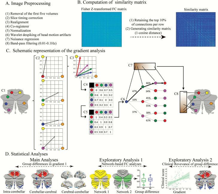
Fig. 1.

Summary of workflow. (A) The steps for image preprocessing. (B and C) Summary of the steps for gradient analysis. Figure 1C adapted from Guell et al³². This example (C1) presents a schematic representation of gradient analysis. It illustrates the calculation of the principal functional gradient of 4 cerebellar voxels (red, green, blue, magenta) based on their functional connectivity with 2 target cerebellar voxels (yellow, orange). (C2) Connectivity from each cerebellar voxel (red, green, blue, magenta) to the 2 target cerebellar voxels (yellow, orange) is represented as a 2-dimensional vector. (C3) All vectors can be represented in the same 2-dimensional space. (C4) Cosine distance between each pair of vectors is calculated, and (C5) an affinity matrix is constructed as (1-cosine distance) for each pair of vectors. This affinity matrix represents the similarity of the connectivity patterns of each pair of voxels. (C6) A Markov chain is constructed using information from the affinity matrix. Information from the affinity matrix is thus used to represent the probability of transition between each pair of vectors. In this way, there will be higher transition probability between pairs of voxels with similar connectivity patterns. This probability of transition between each pair of vectors can be analyzed as a symmetric transformation matrix, thus allowing the calculation of eigenvectors. (C7) Eigenvectors derived from this transformation matrix represent the principal orthogonal directions of transition between all pairs of voxels. Here we illustrate the first resulting component of this analysis – the principal functional gradient of our 4 cerebellar voxels (red, green, blue, magenta) based on their connectivity with our 2 target cerebellar voxels (yellow, orange) progresses from the blue, to the green, to the magenta, to the red voxel. (C8) This order is mapped back into our cerebellum map, allowing us to generate functional neuroanatomical descriptions. Of note, cerebellar functional gradients were calculated using functional connectivity values of each cerebellar voxel with the rest of cerebellar voxels, or each cerebellar voxel with each cerebral cortical voxel, or each cerebral cortical voxel with each cerebellar voxel (rather than between 4 voxels and only 2 target cerebellar voxels, as in this example). Vectors in our analysis thus possessed many more than just two dimensions, but cosine distance can also be calculated between pairs of high-dimensional vectors. (D) Statistical analyses.