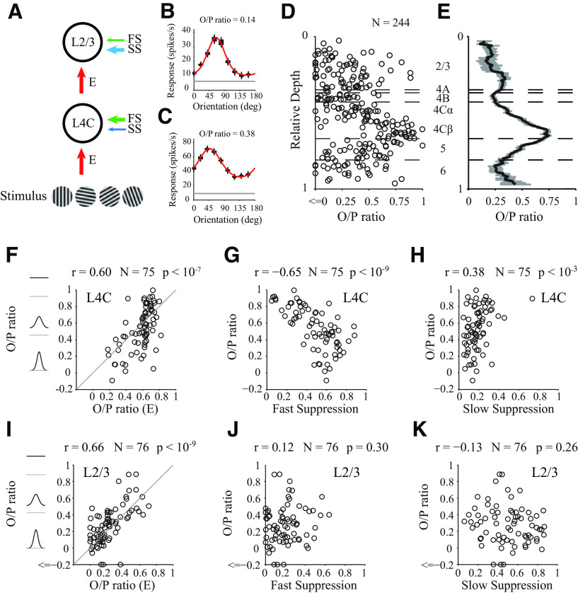
Figure 7.

Correlation of three components with orientation selectivity. A, Schematic of the cascade relationship between input layer (L4C) and output layer (L2/3). Stimuli were drifting sinusoidal gratings with different orientations. Arrow thickness represents the strengths of suppression and excitation. B, C, Examples of individual tuning curves measured by drifting gratings of varying orientation. Red curves indicate fits to the data (black dots) using the von Mises function. Gray line indicates the spontaneous rate of firing. Example site in B located in layer 2/3. Example site in C located in layer 4C. D, Scatter plot of O/P ratio, measured with drifting gratings, against relative depth (N = 244). Horizontal black dashed lines indicate the laminar boundaries. E, Running average of O/P ratio at different cortical depth in D. The length of the sliding window for averaging across depth is 0.1 (relative depth) in cortical space. F–H, Relationship between O/P ratio calculated from tuning curves measured by drifting gratings and different mechanisms dissected from dynamic response (D, O/P ratio of excitation; E, FS; F, SS). Scatter plot for all sites of layer 4C. Strength of suppression defined as averaged strength from 0 to 200 ms. I–K, Similar to F–H, but for all sites of layer 2/3.