. 2020 Sep 1;9:e56603. doi: 10.7554/eLife.56603

Figure 2. Spatio-temporal hierarchy.

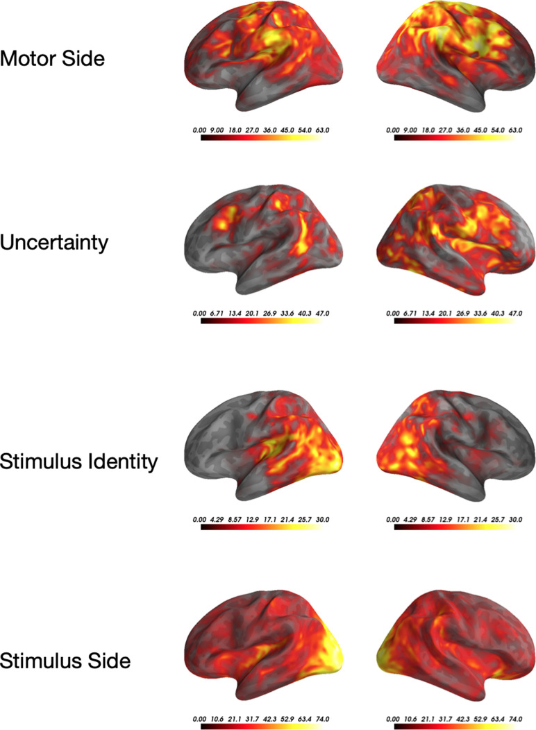
(A) Mass-univariate statistics. Each row plots the average-across-subjects beta coefficients obtained from regression between single-trial evoked activity and each of the five features orthogonally varying in this study. These results are displayed in Video 2. Colors are thresholded based on t-values that exceed an uncorrected p<0.1. We chose this threshold because the perceptual category did not exceed the significance threshold in the univariate tests. (B) Spatial-decoders, consisting of linear models fit across all time sample for each source separately, summarize where each feature can be decoded. Lines indicate significant clusters of decoding scores across subjects cluster-corrected p<0.05. (C) Temporal-decoders, consisting of linear models fit across all MEG channels, for each time sample separately, summarize when each feature can be decoded. To highlight the sequential generation of each representation, decoding scores are normalized by their respective peaks. Additional non-normalized decoding timecourses are available in Figure 2—figure supplements 1 and 2. (D) The peak and the start of temporal decoding plotted for each subject (dot) and for each feature (color). (E) The peak spatial decoding plotted for each subject (dot) and for each feature (color).

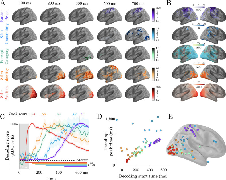
Figure 2.

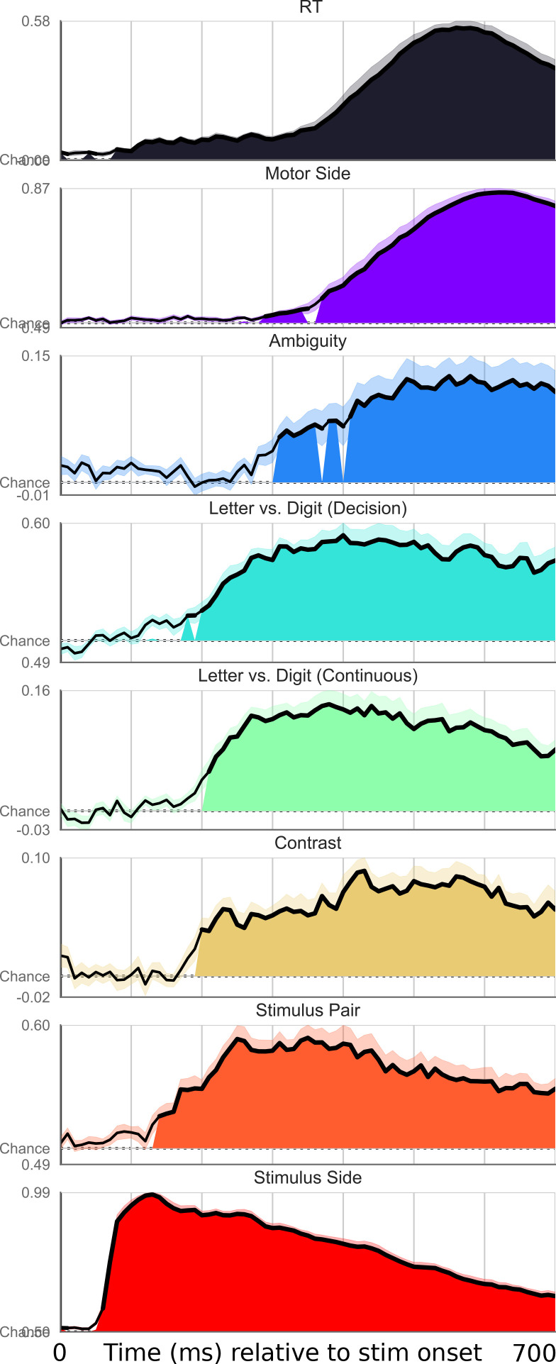
Figure 2—figure supplement 1. Exhaustive set of results for decoding different features of the stimulus, time-locked to stimulus onset.

Figure 2—figure supplement 1.

Shaded area indicates significant decoding as confirmed with a one-sample temporal cluster test.
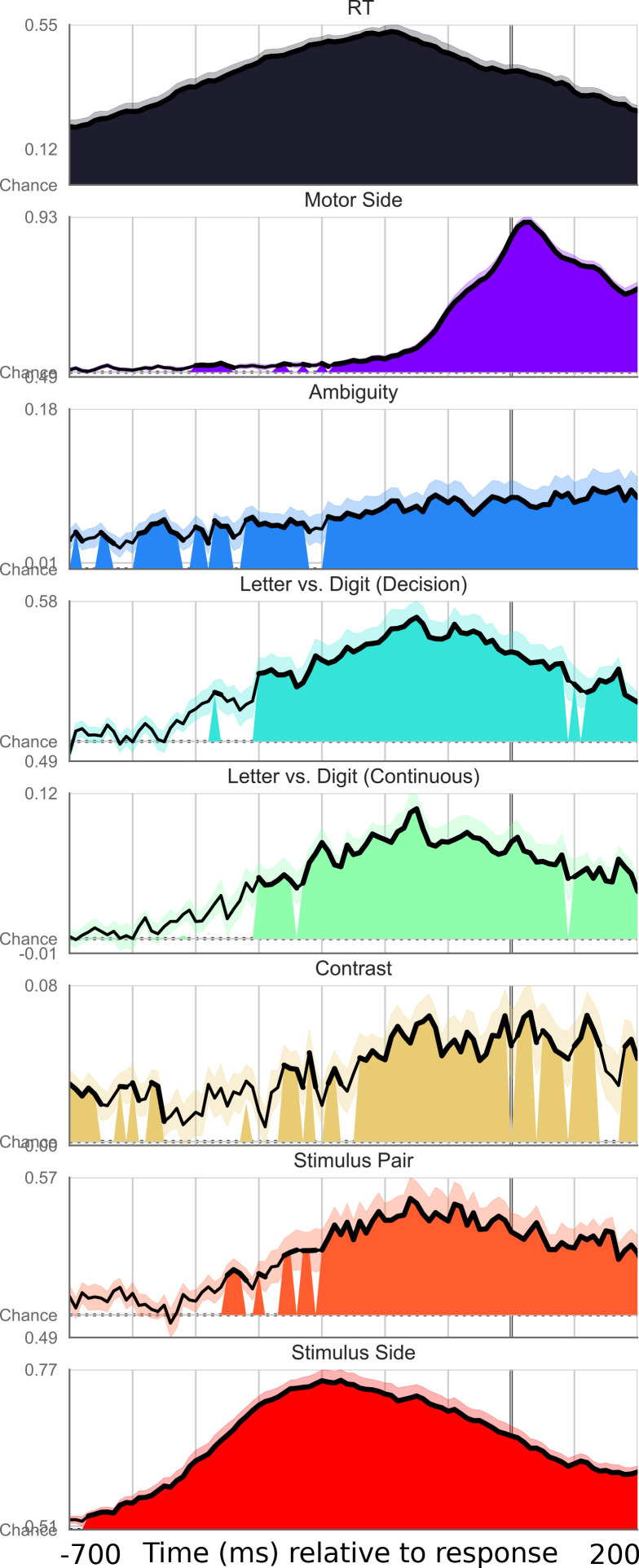
Figure 2—figure supplement 2. Exhaustive set of results for decoding different features of the stimulus, time-locked to motor onset.

Figure 2—figure supplement 2.

Shaded area indicates significant decoding as confirmed with a one-sample temporal cluster test.
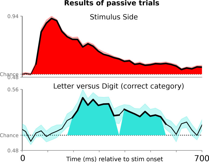
Figure 2—figure supplement 3. Decoding letter/digit contrast for symbols not presented in the active condition, where subjects viewed the symbols passively and did not have to make a motor response.

Figure 2—figure supplement 3.

Figure 2—figure supplement 4. Univariate significance mask for ‘Stimulus Position’.

Figure 2—figure supplement 4.

Localized sources that are contained in a significant (p<0.05) cluster and the specified time-points are highlighted in black.
Figure 2—figure supplement 5. Univariate significance mask for ‘Stimulus Identity’.

Figure 2—figure supplement 5.

Localized sources that are contained in a significant (p<0.05) cluster and the specified time-points are highlighted in black.
Figure 2—figure supplement 6. Univariate significance mask for ‘Uncertainty’.

Figure 2—figure supplement 6.

Localized sources that are contained in a significant (p<0.05) cluster and the specified time-points are highlighted in black.
Figure 2—figure supplement 7. Univariate significance mask for ‘Motor Side’.

Figure 2—figure supplement 7.

Localized sources that are contained in a significant (p<0.05) cluster and the specified time-points are highlighted in black.
Figure 2—figure supplement 8. Univariate significance across the four significant features.

Figure 2—figure supplement 8.

Localized sources that are contained in a significant (p<0.05) cluster. Colormap indicates for how many time-points the vertex was included in a cluster.
Figure 2—figure supplement 9. Significance of multivariate tests across the five significant features.

Figure 2—figure supplement 9.

Localized sources that are contained in a significant (p<0.05) cluster in the spatial decoding analysis.
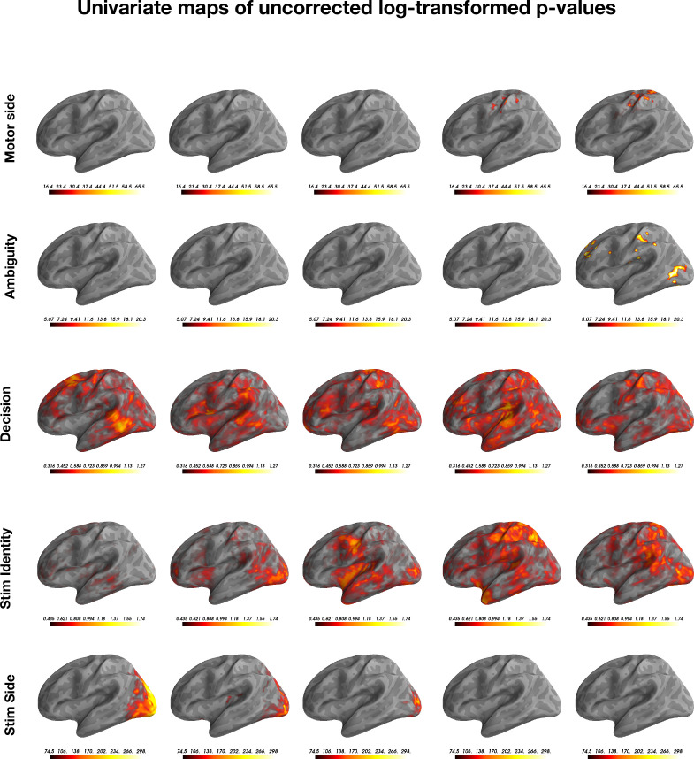
Figure 2—figure supplement 10. Non-corrected log-transformed (base 10) p-values for the mass univariate tests, plotted for each of the five features.

Figure 2—figure supplement 10.

Note that each feature is has a different color-map threshold.
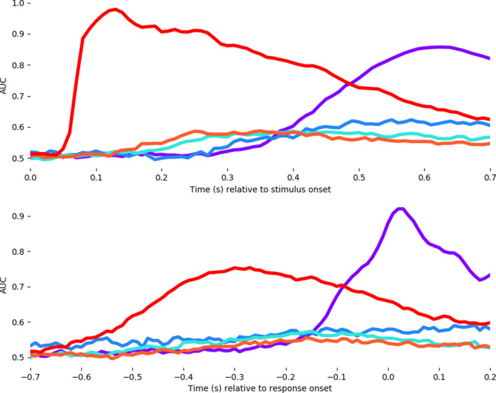
Figure 2—figure supplement 11. Average decoding timecourses for each of the five features.

Figure 2—figure supplement 11.

Timing is locked to stimulus onset (above) and motor response onset (below). Unlike the analysis of Ambiguity (blue line) in the main test, here we median-split the ambiguity variable to fit a logical regression and thus show the AUC values in comparison to the other features.
Figure 2—animation 1. Violin plot of decoding accuracy for the five features of interest over time.
Each dot represents a different subject. The shaded area represents the distribution density of the decoding performance scores across subjects. The dashed black line indicates chance decoding performance for that feature.