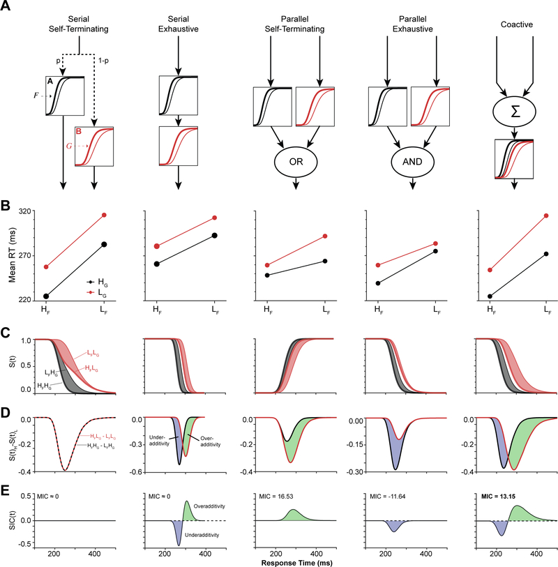
Figure 4.

Systems factorial technology simulations. (A) Each of five processing architectures were modeled using two simple linear accumulator models, each representing an independent operation or stage. The two operations, A and B, were assumed to be under the selective influence of Factors F and G. Stage A varied with Factor F (but not G), and Stage B varied with Factor G (but not F). Essential features of each architecture are shown with depictions of relative stage durations. (B) Mean interaction contrast. Plots of mean RT for each trial type of the double factorial setup. Lines in red and black refer to Low and High levels of Factor G. (C) Survivor function S(t) for each trial type. The gray and red shadings highlight the effects of Factor F on S(t) at fixed levels of Factor G. (D) Difference in survivor function S(t) for fixed levels of Factor G. Regions of blue and green denote intervals of underadditivity and overadditivity, respectively. (E) Survivor interaction contrast S(t). The serial self-terminating architecture produced a SIC that did not differ from 0.0 for all time. The serial exhaustive architecture produced a SIC that deviated to under-additivity followed by over-additivity, with equal area under each region. The parallel self-terminating architecture produced a SIC with overadditivity. The parallel exhaustive architecture produced a SIC with underadditivity. The coactive architecture produced a SIC that deviated to underadditivity followed by overadditivity, with greater area under the overadditive region for net overadditivity.