. 2020 Sep 9;9:e57671. doi: 10.7554/eLife.57671

Figure 6. Vernalization requirement for FLC downregulation is saturated in natural winters.

(A–F) Bolting time for accessions and NILs after transfer to floral-induction conditions from ‘natural’ winter 2016–7, in (A) Norwich 21/10/16 (B) Norwich 21/12/16 (C) South Sweden 01/10/2016 (D) South Sweden 17/12/16 (E) North Sweden 06/09/2016 (F) North Sweden 24/11/2016. Plants that did not flower by 14/02/17 (C, D) or 23/12/16 (E, F) are shown as DNF and dead plants are indicated. Plots show the histogram of numbers of plants as the width of violin plots. A line connects the measurements to indicate the range. Flowering time of genotypes that are significantly different to the reference line Col FRI are indicated by * (ANOVA with Dunnett’s post-hoc test). p-values for all comparisons are given in Supplementary file 3. (G–H) North Sweden 2016 transfers for accessions and NILs, (G) mean time to bolting after transfer to floral-inductive conditions plotted against mean FLC expression per genotype at transfer, Norwich 2016–7, linear regression R2 = 0.68, p<0.001. (H) Mean time to bolting after transfer to floral-inductive conditions plotted against mean FLC expression per genotype at transfer, North Sweden 2016–7. Genotypes that did not bolt within 205 days not shown, linear regression R2 = 0.85, p<0.001. N = 12 plants except where plants died or (E, H) did not bolt within 205 days (Source data 5). Error bars for G and H show s.e.m.

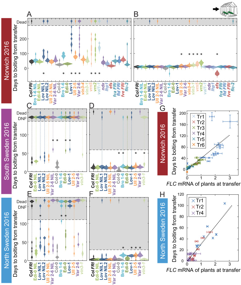
Figure 6.

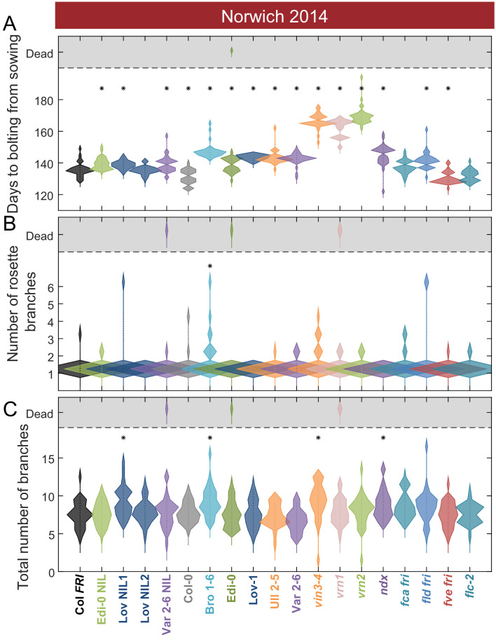
Figure 6—figure supplement 1. Flowering after winter in Norwich 2014–5 in the field was largely synchronous.

Figure 6—figure supplement 1.

(A) Time to bolting for each genotype in the ‘field’ glasshouse in Norwich 2014–5 experiment. (B) Number of rosette branches for plants shown in A. (C) Number of rosette and cauline branches for plants shown in A. Plots A-C show the histogram of numbers of plants as the width of violin plots. A line connects the measurements to indicate the range. N = 36, except where plants did not germinate, Source data 4. Features of genotypes that are significantly different to the reference line Col FRI are indicated by * (ANOVA with Dunnett’s post-hoc). p-values for all comparisons are given in Supplementary file 3.
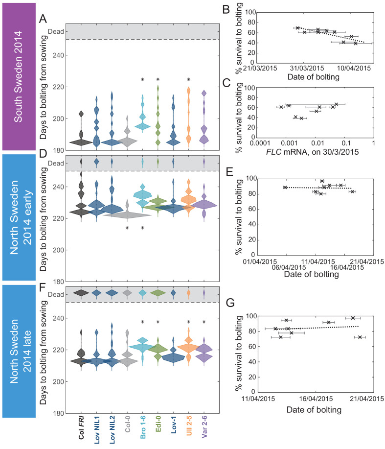
Figure 6—figure supplement 2. The transition to flowering after natural winters in South and North Sweden 2014–5 in the field was largely synchronous, while later bolting had a negative effect on survival only in South Sweden.

Figure 6—figure supplement 2.

(A, D, F) Time to bolting for each genotype, showing the histogram of numbers of plants as the width of violin plots. A line connects the measurements to indicate the range. Flowering time of genotypes that are significantly different to the reference line Col FRI are indicated by * (ANOVA with Dunnett’s post-hoc). p-values for all comparisons are given in Supplementary file 3. (B, E, G) Percentage of germinated plants of each genotype surviving to date of bolting, plotted against the mean date of bolting for that genotype. (B) South Sweden, Generalised Linear Models (GLMs) for binomial distribution, survival vs. date of bolting, p=0.0416. (C) South Sweden, percentage survival vs. mean FLC mRNA per genotype (normalised to control sample for 2014–5) on 30th March, GLM for binomial distribution, ns. (E, G) GLM for binomial distribution, ns. N = 36, except where plants died before flowering, Source data 4. Error bars on scatter plots show s.e.m.
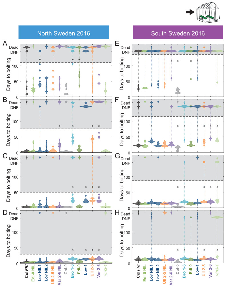
Figure 6—figure supplement 3. Bolting after transfer to warm, long-day conditions from winter in the field 2016–7 saturates at different rates in different genotypes in Sweden.

Figure 6—figure supplement 3.

Bolting time from sequential transfers to long-day warm conditions from the field, for each genotype and transfer. Plots show the histogram of numbers of plants as the width of violin plots. A line connects the measurements to indicate the range. Flowering time of genotypes that are significantly different to the reference line Col FRI are indicated by * (ANOVA with Dunnett’s post-hoc). p-values for all comparisons are given in Supplementary file 3. (A–D) North Sweden, transfer dates: 06/09/2016, 04/10/2016, 01/11/2016, 24/11/2016, experiment ended on 23/12/16. (E–H) South Sweden, transfer dates: 01/10/2016, 22/10/2016, 19/11/2016, 17/12/2016, experiment ended on 14/02/17. N = 12, except where plants died before flowering, Source data 5.
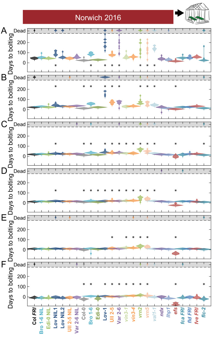
Figure 6—figure supplement 4. Bolting after transfer to warm, long-day conditions from winter in the field 2016–7 saturates at different rates in Norwich.

Figure 6—figure supplement 4.

Bolting from sequential transfers to long-day warm conditions from the field, for each genotype and transfer. The experiment was run until all plants died. Plots show the histogram of numbers of plants as the width of violin plots. A line connects the measurements to indicate the range. Flowering time of genotypes that are significantly different to the reference line Col FRI are indicated by * (ANOVA with Dunnett’s post-hoc). p-values for all comparisons are given in Supplementary file 3. Transfers dates are (A) 21/10/2016, (B) 03/11/2016, (C) 17/11/2016, (D) 30/11/2016, (E) 21/12/2016, (F) 26/01/2017. N = 12, except where plants died before flowering, Source data 5.
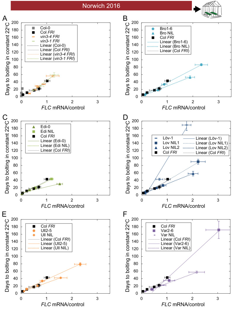
Figure 6—figure supplement 5. The relationship between time to floral transition and FLC expression at the end of cold (Norwich winter 2016–7) varies among accessions, both due to trans effects and due to the FLC alleles themselves.

Figure 6—figure supplement 5.

(A–F) Mean time to bolting of plants moved to a greenhouse lit for 16 hr, and maintained at 22°C/18°C light/dark, plotted against the mean FLC mRNA expression from plants sampled in the Norwich field condition greenhouse on the day of transfer, with linear regression lines plotted for each genotype (the slope ‘m’ being the ‘post-vern’ value, with the y-intercept being the effect on days to bolt if the plants had no detectable FLC, see Table 1). For all accessions and NILs over 3–6 transfers at different times during the winter, R2 = 0.68 for linear regression, p<0.001. N = 6 for expression data, N = 12 for bolting data, except where plants died, Source data 3 and 5. Error bars show s.e.m.
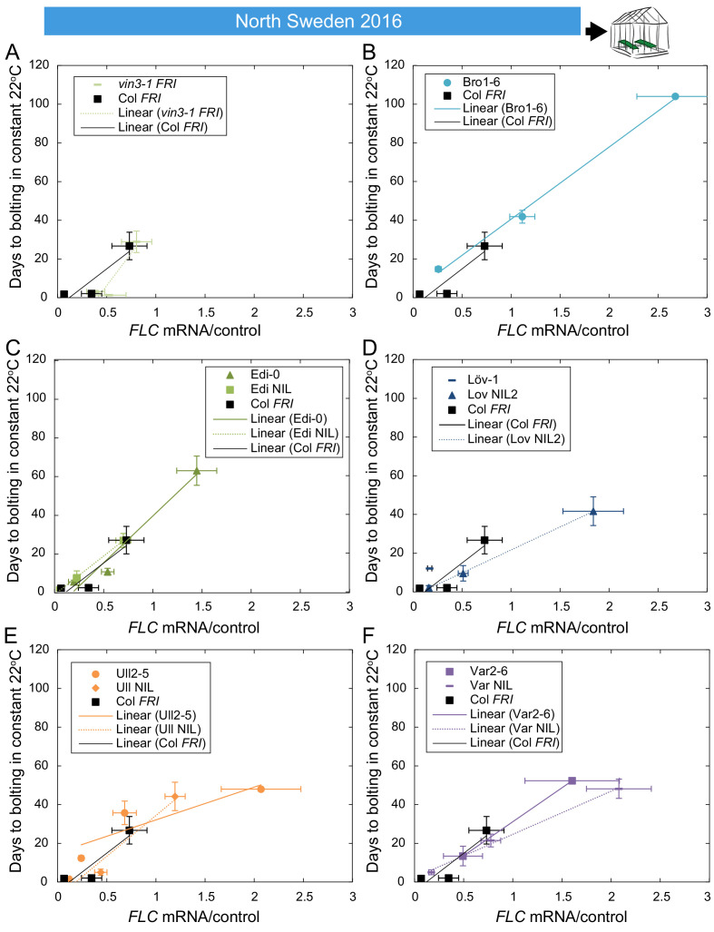
Figure 6—figure supplement 6. The relationship between time to floral transition and FLC expression at the end of cold in North Sweden winter 2016–7.

Figure 6—figure supplement 6.

Mean time to bolting of plants moved to a greenhouse lit for 16 hr, and maintained at 22°C, plotted against the mean FLC mRNA expression from plants sampled in the North Sweden field on or adjacent to the day of transfer, with linear regression lines plotted for each genotype (the slope ‘m’ being the ‘post-vern’ value, with the y-intercept being the effect on days to bolt if the plants had no detectable FLC, see Table 1). (A–F) For all accessions and NILs over 3–6 transfers at different times during the winter, R2 = 0.68 for linear regression, p<0.001. For D, there is no regression for Löv-1 as no Löv-1 plants from the first two transfers flowered within the 120 days of the experiment. N = 12 for bolting data, except where plants died, Source data 3 and 5. Error bars show s.e.m.
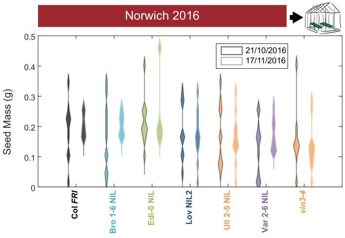
Figure 6—figure supplement 7. Increased vernalization increases the amount and reduces the variability of seed set.

Figure 6—figure supplement 7.

Total seed mass for Col FRI, NILs and the vin3-4 FRI mutant after transfer to floral-induction conditions from ‘natural’ winter in Norwich 2016–7 on 21/10/16 and 17/11/16 (flowering time in Figure 6—figure supplement 4A, C). Plots show the histogram of numbers of plants as the width of violin plots. The time to bolt per plant negatively correlated with seed mass produced, p<0.001, Kenward-Roger’s t-test on REML Linear mixed model with date of transfer as a random factor. N = 12 for transfer 21/10/2016, N = 8–12, mode = 12 for transfer 17/11/2015 due to losses, see Source data 5.