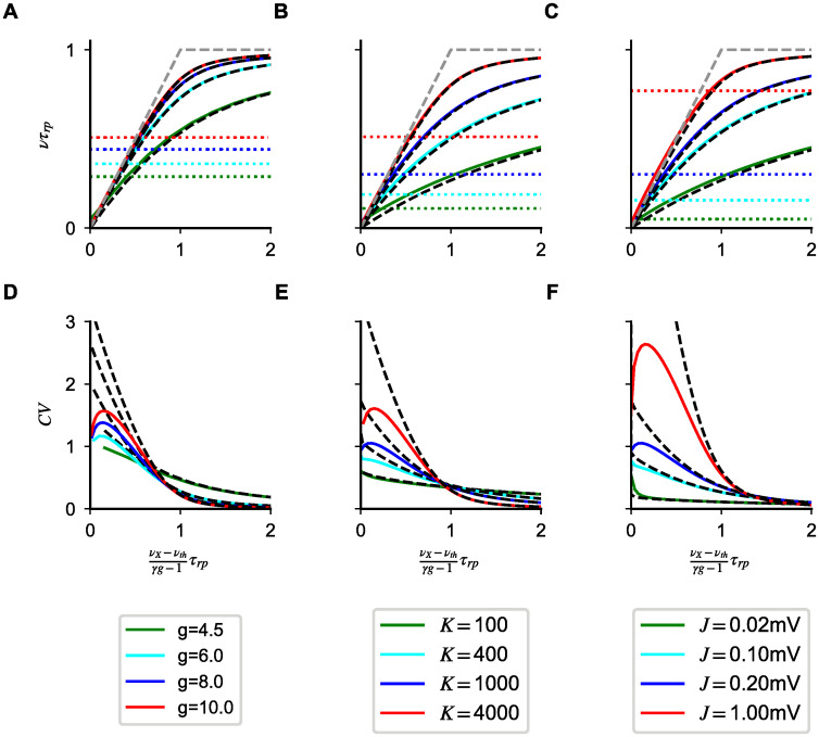
Fig 3. Saturation nonlinearities in Model A.

Transfer function (first row) and CV (second row) computed numerically from Eqs (3)–(5) and (6) (continuous lines) for different g (first column), C (second column) and J (third column). As in Fig 2, colored dotted lines in the first row represent values of the rates at which u_max = − 1. Black dashed lines solutions of the approximated Eqs (13) and (14). This validation of the approximated rate equation motivates the perturbative approach used in the main text and allows to classify nonlinearities in a general way. Simulation parameters: J = 0.2 mV, K = 10³ in (A,D); g = 5.0, J = 0.1mV in (B,E); g = 5.0, K = 10³ in (C,F); in all plots g_X = 1, τ = 20ms.