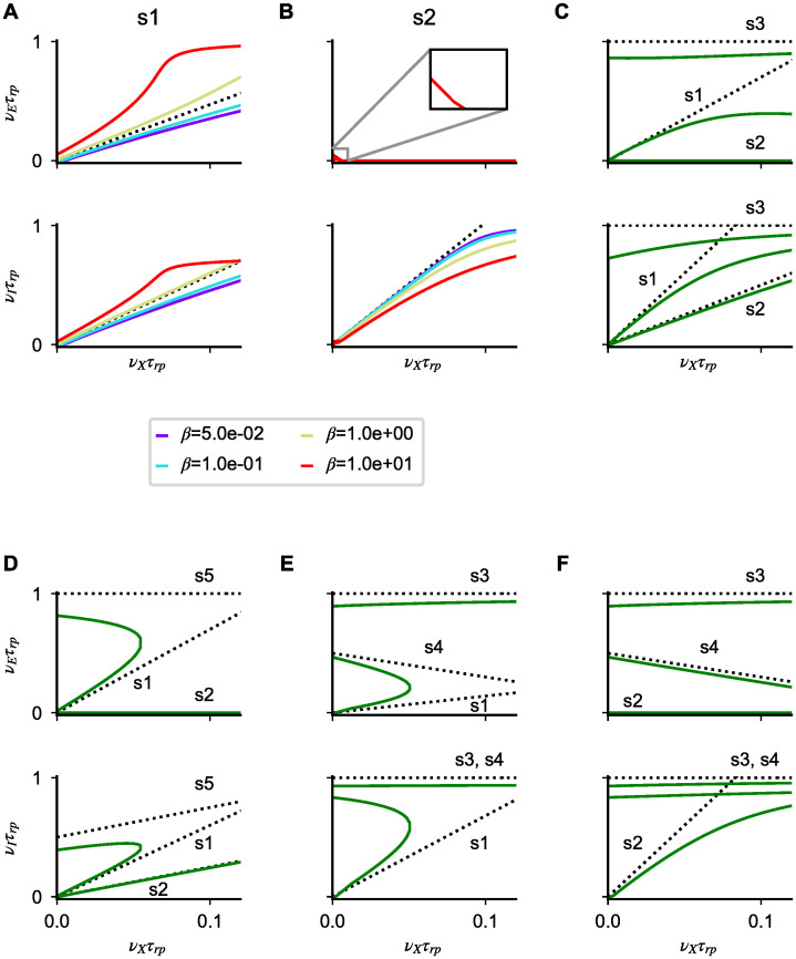
Fig 4. Saturation nonlinearities in model B.
(A-F) Numerical solutions of Eqs (3)–(5) for different parameters (colored lines) and linear approximations predicted by Eqs (24), (26) and (27) in the strong coupling limit (dotted lines). In each panel, the first (second) row shows the excitatory (inhibitory) firing rate as a function of νX. (A,B) Nonlinear solutions obtained at finite coupling starting from solution s1 and s2 for different β values. (C-F) All admissible cases of coexistence of multiple solutions at low νX; note that, as expected from our analysis, the number of solutions changes as νX increases. Simulation parameters are: (A) gI = 3.9, gE = 8, αI = 1 αE = 7; (B) gI = 3.9, gE = 8, αI = 10, αE = 7; (C) gI = 4, gE = 3, αI = 5, αE = 2; (D) gI = 8, gE = 6, αI = 5, αE = 2; (E) gI = 1, gE = 2, αI = 0.3, αE = 2; (F) gI = 1, gE = 2, αI = 3, αE = 2. In panels (A-F), gEX = gIX = 1; JEE = JIE = 0.2mV and KEE = KIE = 103; except in A and B where , .

