COVID-19 pandemic and chaos theory

Abstract

The dynamics of COVID-19 is investigated with regard to complex contributions of the omitted factors. For this purpose, we use a fractional order SEIR model which allows us to calculate the number of infections considering the chaotic contributions into susceptible, exposed, infectious and removed number of individuals. We check our model on Wuhan, China-2019 and South Korea underlying the importance of the chaotic contribution, and then we extend it to Italy and the USA. Results are of great guiding significance to promote evidence-based decisions and policy.

1. Introduction

The coronavirus Covid-19 is affecting almost all the territories around the world, causing viral pneumonia with specific symptomatology [2], [33]. In order to predict the evolution of the Covid-19 pandemic, we have to understand a number of aspects for exploration. We need to know how quickly the viral infection spreads, how long it will last, and more precisely, how quickly it reaches its peak and how quickly it dies. To estimate the epidemic trend, we want to find out the actual steps that we should take in order to control the outbreak and to minimize the damage caused.

Decision-makers face challenges in decisions when dealing with a crisis, therefore an appropriate mathematical model is of great guiding significance to assess the impact of isolation on population. The importance of having a well-organized source of relevant information that gives decision-makers fast, easy and efficient access to the best predictions is essential in order to promote scientific evidence-based decisions and policy goals.

We estimated the number of infections caused by Covid-19, by using SEIR model (Susceptible, Exposed, Infectious, and Removed) [25]. Among many models built to study the amount of the disease spread, SEIR model is one of the most successful [29], [31], [37], [39], [41]. Treatment plays an important role in controlling or decreasing the spread of diseases such as measles, flue and tuberculosis [6], [16], [36]. More recent papers on the effect of treatment on the dynamic behavior of the epidemic SEIR system can be found in [17], [34], [35], [40], [41]. Other more complex models, discussed the global stability of SEIR models with vertical transmission and saturated contact rate [19], [32].

All mathematical models involve simplifications, and it is practically impossible to decide which factors to include and which to omit, and some of the omitted factors are critical. In order to provide quantitative description of all this suppressed contributions, we use fractional calculus. Finding a compact model to describe a complex system is an object of fundamental importance for mathematics. As a generalization of integer order differential equations, fractional calculus has proven to be simple and effective to deal with complex processes.

Sometimes it is hard to distinguish between fractional calculus and chaos theory. The concept of order is associated to the total number of separate differentiations in a system, and it is well-known that chaos cannot occur in continuous systems of total order less than three. However, for a fractional-order system, it is known that this rule is broken and the system can manifest chaotic features [9].

Here, fractional calculus rounds off the exponential nature of solutions given by ordinary differential equations, and provides us a path to realistic behavior of complex systems that we find in the number of infectious persons. After we check our model on the confirmed number of cases in Wuhan, China and on South Korea, we implement it to predict ordinary and chaotic contributions for the epidemic evolution in Italy and the USA.

In analogy with our paper that considered a fractional SEIR model, other papers were published that described fractionally various infectious diseases, using other mathematical models. In [20], the propagation dynamics of infectious diseases on complex networks with a linear treatment function is described using a fractional Susceptible–Infected–Susceptible model. [18] provides a new fractional Susceptible–Infected–Recovered–Susceptible, Susceptible–Infected model that uses the Caputo–Fabrizio fractional operator for the inclusion of memory in order to study the transmission of malaria disease. In [27], in order to study an epidemic model, the authors used a Susceptible–Infected–Recovered model with long-range temporal memory governed by delay fractional-order differential equations.

The paper is organized as follows: in the next section, we introduce some mathematical preliminaries and the Riemann–Liouville fractional integral operator for the generalized fractional-order Bernoulli polynomials, necessary to develop the numerical method used for solve the system of differential equations presented in Section 3. In Section 4, we discuss the spread of infections with and without control measures, taking into account the chaotic behavior.

2. Mathematical model

We start this section with some crucial definitions, the Caputo’s fractional derivative, and the Riemann–Liouville fractional integration.

Definition 2.1

The Caputo’s fractional derivative of order $q$ is defined as [24]

$$\left(D^{q}f\right)\left(x\right)=\frac{1}{\Gamma (n-q)}{\int }_0^x\frac{f^{\left(n\right)}\left(s\right)}{{(x-s)}^{q+1-n}}ds,n-1<q\le n,n\in \mathbb{N},$$ (1)

where $q>0$ is the order of the derivative and $n$ is the smallest integer greater than $q$.

Definition 2.2

The Riemann–Liouville fractional integral operator of order $q$ is defined as [24]

$$I^{q}f\left(x\right)=\left\{\begin{array}{c}\frac{1}{\Gamma \left(q\right)}{\int }_0^x\frac{f\left(s\right)}{{(x-s)}^{1-q}}dsq>0,\hfill \\ f\left(x\right),q=0.\hfill \end{array}\right)$$ (2)

The Caputo derivative and Riemann–Liouville integral satisfy the following properties [26]

$$I^q\left(D^{q}f\left(x\right)\right)=f\left(x\right)-\sum _{k=0}^{n-1}{f}^{\left(k\right)}\left(0\right)\frac{x^k}{k!},$$ (3)

To be able to calculate the Riemann–Liouville fractional integral operator, we need the following representation of the hypergeometric function.

Definition 2.3

The hypergeometric function is defined as

$${}_2{F}_1(a,b,c;z)=\frac{\Gamma \left(c\right)}{\Gamma \left(b\right)\Gamma (c-b)}{\int }_0^1\frac{x^{b-1}{(1-x)}^{c-b-1}}{{(1-xz)}^a}dx.$$

We want to calculate the reliability of our results.

Theorem 2.4

Let $D^{i\alpha }f\left(x\right)\in C(0,1]$ for $i=0,1,\dots ,m$ , then we may formulate the generalized Taylor’s formula [22]

$$f\left(x\right)=\sum _{i=0}^m\frac{x^{i\alpha }}{\Gamma (i\alpha +1)}{D}^{i\alpha }f\left(0^{+}\right)+\frac{x^{m\alpha +\alpha }}{\Gamma (m\alpha +\alpha +1)}{D}^{m\alpha +\alpha }f\left(\xi \right),$$

with $0<\xi \le x$ , $\forall x\in (0,1]$ . Straight computations give

$$|f\left(x\right)-\sum _{i=0}^m\frac{x^{i\alpha }}{\Gamma (i\alpha +1)}{D}^{i\alpha }f\left(0^{+}\right)|\le M_{\alpha }\frac{x^{m\alpha +\alpha }}{\Gamma (m\alpha +\alpha +1)},$$

where $M_{\alpha }={sup}_{\xi \in (0,1]}\left|D^{m\alpha +\alpha }f\left(\xi \right)\right|$ .

Next, we generalize the definition of hybrid functions of block-pulse functions and Bernoulli polynomials by changing the variable $x$ to $x^{\alpha }$, for $\alpha >0$ and then we construct the generalized fractional-order hybrid functions of block-pulse functions and Bernoulli polynomials on the interval $[0,h]$.

Definition 2.5

We define the generalized fractional hybrid function $b_{nm}^{h\alpha }\left(x\right)$, on the interval $[0,h]$ by

$$b_{nm}^{h\alpha }\left(x\right)=\left\{\begin{array}{c}{\beta }_m\left(N\frac{x^{\alpha }}{h^{\alpha }}-n+1\right),x\in \left[h{\left(\frac{n-1}{N}\right)}^{1∕\alpha },h{\left(\frac{n}{N}\right)}^{1∕\alpha }\right),\hfill \\ 0,\mathrm{otherwise},\hfill \end{array}\right)$$ (4)

The generalized fractional-order Bernoulli functions can be defined by

$${\beta }_m^{h\alpha }\left(x\right)=\sum _{k=0}^m\left(\begin{array}{c}\hfill m\hfill \\ \hfill k\hfill \end{array}\right){\alpha }_{m-k}\frac{x^{k\alpha }}{h^{k\alpha }},0\le x\le h,$$ (5)

where ${\alpha }_k$, $k=\overline{1,m}$ are the Bernoulli numbers. The first few generalized fractional-order Bernoulli functions are

$${\beta }_0^{h\alpha }\left(x\right)=1,{\beta }_1^{h\alpha }\left(x\right)=\frac{x^{\alpha }}{h^{\alpha }}-\frac{1}{2},{\beta }_2^{h\alpha }\left(x\right)=\frac{x^{2\alpha }}{h^{2\alpha }}-\frac{x^{\alpha }}{h^{\alpha }}+\frac{1}{6}.$$

For numerical reasons, we make certain approximations.

Definition 2.6

Let $f\in L^2[0,h]$, the best approximation of $f$ by using hybrid functions is given by

$$f\left(x\right)\approx \sum _{m=0}^M\sum _{n=1}^N{c}_{nm}{b}_{nm}^{h\alpha }\left(x\right)=C^{\mathrm{T}}{B}^{h\alpha }\left(x\right),$$ (6)

where

$$C={[c_{10},\dots ,c_{N0},c_{11},\dots ,c_{N1},\dots ,c_{1M},\dots ,c_{NM}]}^{\mathrm{T}},$$

where

$$B^{h\alpha }\left(x\right)={[b_{10}^{h\alpha }\left(x\right),\dots ,b_{N0}^{h\alpha }\left(x\right),b_{11}^{h\alpha }\left(x\right),\dots ,b_{N1}^{h\alpha }\left(x\right),\dots ,b_{1M}^{h\alpha }\left(x\right),\dots ,b_{NM}^{h\alpha }\left(x\right)]}^{\mathrm{T}}.$$

We now derive the Riemann–Liouville fractional integral operator $I^{\beta }$ for the generalized fractional-order Bernoulli polynomials $B^{h\alpha }\left(x\right)$.

Let

$$I^{\beta }{B}^{h\alpha }\left(x\right)\equiv {\overline{B}}^{h\alpha }(x,\beta ),$$ (7)

where

$${\overline{B}}^{h\alpha }(x,\beta )=[I^{\beta }{b}_{10}^{h\alpha }\left(x\right),\dots ,I^{\beta }{b}_{N0}^{h\alpha }\left(x\right),I^{\beta }{b}_{11}^{h\alpha }\left(x\right),\dots ,I^{\beta }{b}_{N1}^{h\alpha }\left(x\right),\dots ,I^{\beta }{b}_{NM}^{h\alpha }\left(x\right)]{}^T.$$

Theorem 2.7

Making the notation $\tilde{N}=\frac{N}{h^{\alpha }}$ , we get the following result

$$I^{\beta }{b}_{nm}^{h\alpha }\left(x\right)=\left\{\begin{array}{c}0,x\in \left(-\infty ,h{\left(\frac{n-1}{N}\right)}^{1∕\alpha }\right),\hfill \\ U\left(x\right),x\in \left[h{\left(\frac{n-1}{N}\right)}^{1∕\alpha },h{\left(\frac{n}{\tilde{N}}\right)}^{1∕\alpha }\right),\hfill \\ U\left(x\right)-V\left(x\right),x\in \left[h{\left(\frac{n}{N}\right)}^{1∕\alpha },\infty \right),\hfill \end{array}\right)$$ (8)

with

$$U\left(x\right)=\sum _{k=0}^m\sum _{r=0}^k\left(\begin{array}{c}\hfill m\hfill \\ \hfill k\hfill \end{array}\right)\left(\begin{array}{c}\hfill k\hfill \\ \hfill r\hfill \end{array}\right){\alpha }_{m-k}{\tilde{N}}^r{(1-n)}^{k-r}\times \left[x^{\alpha r+\beta }\frac{\Gamma (\alpha r+1)}{\Gamma (\beta +\alpha r+1)}-\frac{x^{\beta -1}}{\Gamma \left(\beta \right)(\alpha r+1)}{\left(\frac{n-1}{\tilde{N}}\right)}^{(\alpha r+1)∕\alpha }\right)\times \left({}_2{F}_1\left(1-\beta ,\alpha r+1,\alpha r+2;\frac{1}{x}{\left(\frac{n-1}{\tilde{N}}\right)}^{1∕\alpha }\right)\right],$$

and

$$V\left(x\right)=\sum _{k=0}^m\sum _{r=0}^k\left(\begin{array}{c}\hfill m\hfill \\ \hfill k\hfill \end{array}\right)\left(\begin{array}{c}\hfill k\hfill \\ \hfill r\hfill \end{array}\right){\alpha }_{m-k}{\tilde{N}}^r{(1-n)}^{k-r}\left[x^{\alpha r+\beta }\frac{\Gamma (\alpha r+1)}{\Gamma (\beta +\alpha r+1)}\right)-\left(\frac{x^{\beta -1}}{\Gamma \left(\beta \right)(\alpha r+1)}{\left(\frac{n}{\tilde{N}}\right)}^{(\alpha r+1)∕\alpha }{}_2{F}_1\left(1-\beta ,\alpha r+1,\alpha r+2;\frac{1}{x}{\left(\frac{n}{\tilde{N}}\right)}^{1∕\alpha }\right)\right].$$

Proof

From Eq. (4), we have

$$b_{nm}^{h\alpha }\left(x\right)=\beta \left(\tilde{N}{x}^{\alpha }-n+1\right)\left({\mu }_{{\left(\frac{n-1}{\tilde{N}}\right)}^{1∕\alpha }}\left(x\right)-{\mu }_{{\left(\frac{n}{\tilde{N}}\right)}^{1∕\alpha }}\left(x\right)\right),$$

where ${\mu }_c$ is the unit step function defined as

$${\mu }_c\left(x\right)=\left\{\begin{array}{c}1,x\ge c,\hfill \\ 0,x<c.\hfill \end{array}\right)$$

Applying the definition from Eq. (5), we obtain

$$b_{nm}^{h\alpha }\left(x\right)=\sum _{k=0}^m\sum _{r=0}^k\left(\begin{array}{c}\hfill m\hfill \\ \hfill k\hfill \end{array}\right)\left(\begin{array}{c}\hfill k\hfill \\ \hfill r\hfill \end{array}\right){\alpha }_{m-k}{\tilde{N}}^r{x}^{r\alpha }{(1-n)}^{k-r}$$ (9)

$$\times \left({\mu }_{{\left(\frac{n-1}{\tilde{N}}\right)}^{1∕\alpha }}\left(x\right)-{\mu }_{{\left(\frac{n}{\tilde{N}}\right)}^{1∕\alpha }}\left(x\right)\right).$$

By applying the Riemann–Liouville integral operator to Eq. (9) we obtain

$$I^{\beta }{b}_{nm}^{h\alpha }\left(x\right)=\sum _{k=0}^m\sum _{r=0}^k\left(\begin{array}{c}\hfill m\hfill \\ \hfill k\hfill \end{array}\right)\left(\begin{array}{c}\hfill k\hfill \\ \hfill r\hfill \end{array}\right){\alpha }_{m-k}{\tilde{N}}^r{(1-n)}^{k-r}\times \left(I^{\beta }\left(x^{\alpha r}{\mu }_{{\left(\frac{n-1}{\tilde{N}}\right)}^{1∕\alpha }}\left(x\right)\right)-I^{\beta }\left(x^{\alpha r}{\mu }_{{\left(\frac{n}{\tilde{N}}\right)}^{1∕\alpha }}\left(x\right)\right)\right).$$ (10)

Using the representation (4), we obtain

$$I^{\beta }\left(x^{\alpha }{\mu }_c\left(x\right)\right)=x^{\alpha +\beta }\frac{\Gamma (\alpha +1)}{\Gamma (\beta +\alpha +1)}-\frac{x^{\beta -1}}{\Gamma \left(\beta \right)}\frac{c^{\alpha +1}}{\alpha +1}{}_2{F}_1\left(1-\beta ,\alpha +1,\alpha +2;\frac{c}{x}\right),$$

and the theorem is proved by introducing this result in Eq. (10). □

The following Theorem gives the error bound of the approximate solution.

Theorem 2.8

Suppose that $D^{i\alpha }\in C(0,h]$ for $i\in \overline{0,M}$ , $(\hat{m}=N(M+1))$ and $Y_{\hat{m}}^{h\alpha }=\{{\beta }_0^{h\alpha }\left(x\right),{\beta }_1^{h\alpha }\left(x\right),\dots {\beta }_{M-1}^{h\alpha }\left(x\right)\}$ . If $f_M\left(x\right)$ is the best approximation of $f\left(x\right)$ out of $Y_{\hat{m}}^{h\alpha }$ on the interval $\left[h{\left(\frac{n-1}{N}\right)}^{1∕\alpha },h{\left(\frac{n}{N}\right)}^{1∕\alpha }\right]$ , then the error bound of the approximate solution $f_{\hat{m}}\left(x\right)$ by using the fractional-order hybrid functions of block-pulse and Bernoulli polynomials on the interval $[0,h]$ would be obtained as follows

$${\Vert f-f_{\hat{m}}\Vert }_{L^2[0,h]}\le \frac{\sqrt{h}\underset{x\in [0,h]}{sup}\left|D^{M\alpha +\alpha }f(x∕h)\right|}{\Gamma (M\alpha +\alpha +1)\sqrt{2M\alpha +2\alpha +1}}.$$ (11)

Proof

We define

$$f_1\left(x\right)=\sum _{i=0}^M\frac{{(x∕h)}^{i\alpha }}{\Gamma (i\alpha +1)}{D}^{i\alpha }f\left(0^{+}\right).$$

From the generalized Taylor’s formula defined in Theorem 2.4, we have

$$|f\left(x\right)-f_1\left(x\right)|\le \frac{{(x∕h)}^{M\alpha +\alpha }}{\Gamma (M\alpha +\alpha +1)}\underset{x\in I_n^{h\alpha }}{sup}\left|D^{M\alpha +\alpha }f(x∕h)\right|,$$

where $I_n^{h\alpha }=\left[h{\left(\frac{n-1}{N}\right)}^{1∕\alpha },h{\left(\frac{n}{N}\right)}^{1∕\alpha }\right)$.

Since $f_M\left(x\right)$ is the best approximation of $f\left(x\right)$ out of $Y_m^{h\alpha }$ on the interval $I_n^{h\alpha }$ and $f_1\left(x\right)\in Y_m^{h\alpha }$, one may write

$${\Vert f-f_{\hat{m}}\Vert }_{L^2[0,h]}^2$$ (12)

$$\le \sum _{n=1}^N{\Vert f-f_M\Vert }_{L^2{I}_n^{h\alpha }}^2\le \sum _{n=1}^N{\Vert f-f_1\Vert }_{L^2{I}_n^{h\alpha }}^2\le \sum _{n=1}^N{\int }_{I_n^{h\alpha }}{\left[\frac{{(x∕h)}^{M\alpha +\alpha }}{\Gamma (M\alpha +\alpha +1)}\underset{x\in I_n^{h\alpha }}{sup}\left|D^{M\alpha +\alpha }f(x∕h)\right|\right]}^{2}dx\le {\int }_0^h{\left[\frac{{(x∕h)}^{M\alpha +\alpha }}{\Gamma (M\alpha +\alpha +1)}\underset{x\in [0,h]}{sup}\left|D^{M\alpha +\alpha }f(x∕h)\right|\right]}^{2}dx\le \frac{h}{\Gamma {(M\alpha +\alpha +1)}^2(2M\alpha +2\alpha +1)}{\left(\underset{x\in [0,h]}{sup}\left|D^{M\alpha +\alpha }f(x∕h)\right|\right)}^2.$$

The theorem is proved by taking the square roots.

In the above Theorem we have defined $I_n^{\alpha }=\left({\left(\frac{n-1}{N}\right)}^{1∕\alpha },{\left(\frac{n}{N}\right)}^{1∕\alpha }\right]$. When $M$ is fixed and $N$ approaches $\infty$, we have

$$\left|I_n^{\alpha }\right|=|{\left(\frac{n-1}{N}\right)}^{1∕\alpha }-{\left(\frac{n}{N}\right)}^{1∕\alpha }|\to 0,$$

which yields

$$\underset{N\to \infty }{lim}{\Vert f-f_{\hat{m}}\Vert }_{L^2[0,h]}=0.$$

We see from Eq. (11) that the limit $M\to \infty$ gives

$$\underset{M\to \infty }{lim}{\Vert f-f_{\hat{m}}\Vert }_{L^2[0,h]}=0.$$

3. The numerical method

This paper is build on a fractional order extension of the SEIR model. This model simulates the spread of pathogens, and is based on the compartmentalization of people in four classes: susceptible $S$, exposed $E$, infectious $I$ and recovered $R$. The predictions are made to see how these compartments change over time. The fractional-order differential equations of the SEIR model are defined as [3], [4]

$$\left\{\begin{array}{ccc}{D}^{a}S\left(x\right)\hfill & =\hfill & -\frac{\beta }{N}S\left(x\right)I\left(x\right),\hfill \\ D^{b}E\left(x\right)\hfill & =\hfill & \frac{\beta }{N}S\left(x\right)I\left(x\right)-\sigma E\left(t\right),\hfill \\ D^{c}I\left(x\right)\hfill & =\hfill & \sigma E\left(x\right)-\gamma I\left(x\right),\hfill \\ D^{d}R\left(x\right)\hfill & =\hfill & \gamma I\left(x\right),\hfill \end{array}\right)$$ (13)

$a$, $b$, $c$, $d\in (0,2]$. $S$ represents the class of susceptible individuals, and in this paper, the disease can be transmitted from any infected individual to any susceptible one. The class of exposed individuals $E$ is composed of individuals who are directly exposed to the infected disease but are not infectious. $I$ defines the class of infectious individuals, and by definition, any infectious person can transmit the disease. Anyone who was previously infectious and is no longer infectious (recovered or dead) form the class of recovered individuals $R$. The population sample $N$ to be analyzed is defined by $N=S+E+I+R$. $\beta$ is the average number of interactions per person per time, multiplied by the probability of transmission at each interaction between a susceptible and an infected individual, $\gamma$ is the transition rate at which and infected individual moves to the recovered class, $\sigma$ is the rate at which exposed individuals become infectious and $R_0$ the basic reproduction number.

Throughout the paper, we are interested how the number of infections is influenced by the number of susceptible, exposed, and removed individuals. Here, we solve this problem with $a=\theta$, $b=\eta$, $c=\lambda$ and $d=\delta$, by using the hybrid functions with $N=2$ and $M=15$. We are expanding $D^{a}S\left(t\right),D^{b}E\left(t\right),D^{c}I\left(t\right)$ and $D^{d}R\left(t\right)$ into fractional-order hybrid functions as

$$\left\{\begin{array}{ccc}{D}^{a}S\left(x\right)\hfill & =\hfill & C_1^T{B}^{h\theta }\left(x\right),\hfill \\ D^{b}E\left(x\right)\hfill & =\hfill & C_2^T{B}^{h\eta }\left(x\right),\hfill \\ D^{c}I\left(x\right)\hfill & =\hfill & C_3^T{B}^{h\lambda }\left(x\right),\hfill \\ D^{d}R\left(x\right)\hfill & =\hfill & C_4^T{B}^{h\delta }\left(x\right),\hfill \end{array}\right)$$ (14)

and using this result together with Eqs. (3), (14), one gets the following system of algebraic equations

$$\left\{\begin{array}{ccc}S\left(x\right)\hfill & =\hfill & C_1^T{\overline{B}}^{h\theta }(x,a)+S\left(0\right),\hfill \\ E\left(x\right)\hfill & =\hfill & C_2^T{\overline{B}}^{h\eta }(x,b)+E\left(0\right),\hfill \\ I\left(x\right)\hfill & =\hfill & C_3^T{\overline{B}}^{h\lambda }(x,c)+I\left(0\right),\hfill \\ R\left(x\right)\hfill & =\hfill & C_4^T{\overline{B}}^{h\delta }(x,d)+R\left(0\right).\hfill \end{array}\right)$$ (15)

By substituting Eqs. (15), (14) into Eq. (13), we obtain

$$\left\{\begin{array}{ccc}{C}_1^T{B}^{h\theta }\left(x\right)\hfill & =\hfill & -\frac{\beta }{N}(C_1^T{\overline{B}}^{h\theta }(x,a)+S\left(0\right))(C_3^T{\overline{B}}^{h\lambda }(x,c)+I\left(0\right)),\hfill \\ C_2^T{B}^{h\eta }\left(x\right)\hfill & =\hfill & \frac{\beta }{N}(C_1^T{\overline{B}}^{h\theta }(x,a)+S\left(0\right))(C_3^T{\overline{B}}^{h\lambda }(x,c)+I\left(0\right))\hfill \\ \hfill & \hfill & -\sigma (C_2^T{\overline{B}}^{h\eta }(x,b)+E\left(0\right)),\hfill \\ C_3^T{B}^{h\lambda }\left(x\right)\hfill & =\hfill & \sigma (C_2^T{\overline{B}}^{h\eta }(x,b)+E\left(0\right))-\gamma (C_3^T{\overline{B}}^{h\lambda }(x,c)+I\left(0\right)),\hfill \\ C_4^T{B}^{h\delta }\left(x\right)\hfill & =\hfill & \gamma (C_3^T{\overline{B}}^{h\lambda }(x,c)+I\left(0\right)).\hfill \end{array}\right)$$

Next, we collocate these equations in the Newton–Cotes nodes $x_i$ given by

$$x_i=h{\left(\frac{i+1}{2N(M+1)}\right)}^{1∕\alpha },i=0,1,\dots ,2N(M+1)-2.$$

These equations give $\hat{m}=N(M+1)$ algebraic equations, which can be solved for the unknown vectors $C_1$, $C_2$, $C_3$ and $C_4$, using Newton’s iterative method. Introducing this vector into Eq. (14), one gets the approximation of order $\hat{m}$ for the function $I\left(x\right)$.

Definition 3.1

If the exact solution of the problem is not known, in order to test the reliability of the results one should introduce the residual error function [38]

$$R_h=\underset{x\in [0,h]}{max}|D^{c}I\left(x\right)-\sigma E\left(x\right)+\gamma I\left(x\right)|.$$

The reliability in our numerical computation is about 1%. In order to decrease this percent, we should increase $N$ and $M$ in Eq. (14).

4. Discussion

The SEIR model, has been used successfully in the description of some infectious disease as Ebola and SARS [1], [5], [7], [8], [23], [28], [30]. For our purposes, we assumed no transmissions from animals and no differences in natural births and deaths. Besides, we consider no maternal immunity and we ask that all recovered individuals acquire permanent immunity [21]. In the construction of the classical model, we do not know if we have super-spreaders behavior and we do not really know the accuracy of the incubation period. Moreover, $R_0$ is essentially a dynamic parameter. In order to include all these contributions, we apply fractional calculus.

Using this information and the data provided by [10] we can assign start and end dates for each epidemic phase. The reproduction number $R_0$ is assigned for each phase based on the prevention measures of each country and how probable is that people will respect said measures.

In the first part of this paper, we check our model by comparing it with the model described in [33] for estimating the number of coronavirus disease 2019 cases in Wuhan, China, and after that, we introduce the chaotic contribution. Thus, we consider the system of fractional differential equations described in Eqs. (13), subject to the initial conditions $S\left(0\right)=11000000$, $E\left(0\right)=800$, $I\left(0\right)=40$, and $R\left(0\right)=0$, with the setup $\beta =R_0∕\gamma$, $\sigma =1∕5.2$, $\gamma =1∕18$, $R_0=2.6$, $N=1100840$.

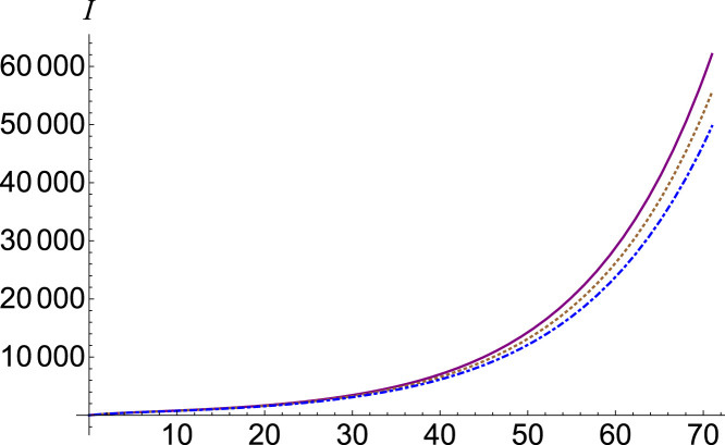
To understand the chaotic contribution to the number of infections, we adjust the parameter $c$ in the system of Eqs. (13). The function $I$ has a very strong dependency over the parameter $c$. This effect can be seen in Fig. 1, where we plotted the number of infections $I$, $c=\lambda =1$ (purple, continuous), $c=\lambda =0.99$ (brown, dotted) and $c=\lambda =0.98$ (blue, dot-dashed). $c\ne 1$ means the contribution of critical omitted factors to the number of infections. If we consider $c\in (1,2]$, then we have a positive contribution.

Fig. 1.

Infected number $I$, $c=\lambda =1$ (purple, continuous), $c=\lambda =0.99$ (brown, dotted) and $c=\lambda =0.98$ (blue, dot-dashed).

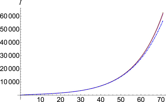
In order to study the chaotic contribution of the number of susceptible individuals in the number of infected ones, we adjust the parameter $a$. In Fig. 2, we see that the function dependency on the parameter $a$ is very weak. The setting is $a=\theta =1$ (purple, continuous), $a=\theta =0.1$ (brown, dotted) and $a=\theta =1.8$ (blue, dot-dashed).

Fig. 2.

Infected number $I$, $a=\theta =1$ (purple, continuous), $a=\theta =0.1$ (brown, dotted) and $a=\theta =1.8$ (blue, dot-dashed).

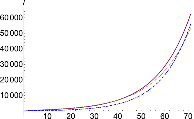
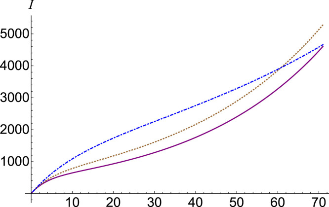
If we are interested in the chaotic contribution of the number of exposed individuals on the number of infected ones, we have to adjust the parameter $b$. The function $I$ has a smaller dependency compared to the parameter $c$. When $b\in (0,1]$ the number of infected people decreases, and when $b\in (1,2]$, for small $b$ the number of infected people increases slightly, and then begins to decrease. This behavior is represented in Fig. 3, where we plotted the number of infections $I$, $b=\eta =1$ (purple, continuous), $b=\eta =0.9$ (brown, dotted) and $b=\eta =1.3$ (blue, dot-dashed) for $R_0=1.3$. A clearer growth behavior followed by decline can be seen in Fig. 4, where we plotted $I$ with $b=\eta =1$ (purple, continuous), $b=\eta =0.9$ (brown, dotted) and $b=\eta =1.3$ (blue, dot-dashed) for $R_0=1.8$.

Fig. 3.

Infected number $I$, $b=\eta =1$ (purple, continuous), $b=\eta =0.9$ (brown, dotted) and $b=\eta =1.3$ (blue, dot-dashed).

Fig. 4.

Infected number $I$, $b=\eta =1$ (purple, continuous), $b=\eta =0.9$ (brown, dotted) and $b=\eta =0.5$ (blue, dot-dashed), for $R_0=1.8$.

The number of recovered individuals $R$ in the system of Eqs. (13), is independent on the first three equations, therefore $d$ variations have no influence over $I$. Due to a very weak dependence, in our further analysis we can neglect the contribution of the parameter $a$.

Next step in the epidemic analysis is to anticipate the numbers of the infectious assuming an ensemble of prevention and control measures imposed by each country in phases. Each phase is characterized by a basic reproduction numbers $R_0$. We should mention two behavior of this parameter: when $R_0>0$ we have a self-sustaining situation, otherwise, the number of new cases decreases, and eventually the outbreak will stop.

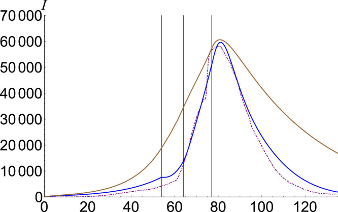
In Fig. 5 we plot in brown our ordinary estimation $I$ for China on the interval 1 December $2019--23$ April 2020 and we compare it to the number of confirmed cases in purple. Each phase [12] is described in Table 1, and in Fig. 5 is delimited by a vertical line. To make a better estimation, we fit our fractional model with $c_1={\lambda }_1=0.9$, $c_2={\lambda }_2=1.3$, $c_3={\lambda }_3=1.35$, $c_4={\lambda }_4=1.15$ and $b_4={\eta }_4=1.3$, where $i=\overline{1,4}$ from $c_i$ represents the phase number, and the result is represented in blue. All other undeclared parameters are considered $1$. The advantages of our presented model are indisputable, improving the estimation by several thousand cases.

Fig. 5.

Infected number $I$ for China. Data is plotted with purple, SEIR solution with brown, and the fractional model $c_1={\lambda }_1=0.9$, $c_2={\lambda }_2=1.3$, $c_3={\lambda }_3=1.35$, $c_4={\lambda }_4=1.15$ and $b_4={\eta }_4=1.3$ with blue.(For interpretation of the references to color in this figure legend, the reader is referred to the web version of this article.)

Table 1.

Phases distribution and the corresponding basic reproduction numbers $R_0$.

Phase	Data	China	South Korea	Italy	USA
1	From	1 Dec 19	9 Feb 20	15 Feb 20	4 Feb 20
	To	23 Jan 20	25 Feb 20	4 Apr 20	4 Apr 20
$R_0$		3.1	4	3.5	3.8
2	From	24 Jan 20	26 Feb 20	5 Apr 20	5 Apr 20
	To	2 Feb 20	1 Mar 20	10 Apr 20	13 Apr 20
$R_0$		2.6	3.5	2.4	3
3	From	3 Feb 20	2 Mar 20	11 Apr 20	14 Apr 20
	To	15 Feb 20	12 Mar 20	28 Apr 20	3 May 20
$R_0$		1.9	2.3	1.3	1.7
4	From	16 Feb 20	13 Mar 20	29 Apr 20	4 May 20
	To	–	–	–	–
$R_0$		0.5	0.5	0.7	0.6

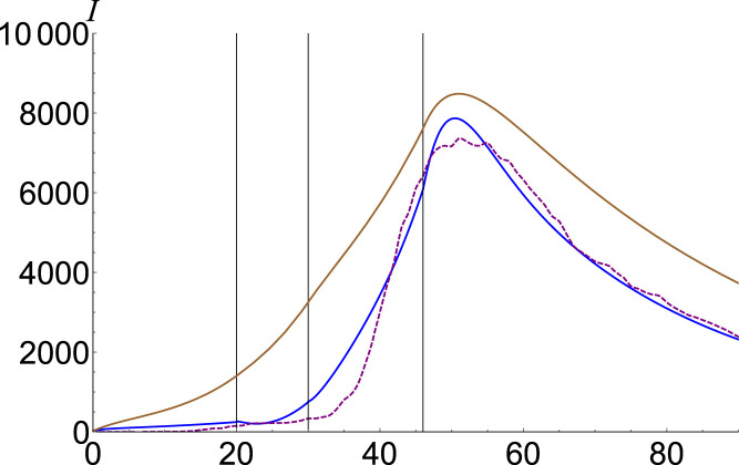
As in the case of China, in Fig. 6 we plot in brown our ordinary estimation $I$ for South Korea on the interval 9 February $2020--23$ April 2020 and we compare it to the number of confirmed cases in purple. Each phase [13] is described in Table 1. To make a better estimation, we fit in blue our fractional model with $c_1={\lambda }_1=0.7$, $c_2={\lambda }_2=1.2$, $c_3={\lambda }_3=1.35$, $c_4={\lambda }_4=1.05$ and $b_4={\eta }_4=1.2$.

Fig. 6.

Infected number $I$ for South Korea. Data is plotted with purple, SEIR solution with brown, and the fractional model $c_1={\lambda }_1=0.7$, $c_2={\lambda }_2=1.2$, $c_3={\lambda }_3=1.35$, $c_4={\lambda }_4=1.05$ and $b_4={\eta }_4=1.2$ with blue.(For interpretation of the references to color in this figure legend, the reader is referred to the web version of this article.)

The ordinary infections described by SEIR is overestimated in the first few phases, and this overestimation is transferred to the last phase. Fractional computation is adjusting the first phases, leading to realistic behavior in prediction. $R_0$ is highly unknown, especially in the first phases, and in order to get the real data characteristics we should artificially decrease $I$, by imposing $c_1<1$. To balance the results and hit the peak, we should make it bigger than $1$ in both second and third phases. Due to the magnification of the infectious persons, we raise the contribution of the exposed, and in the last phase one should adjust it asking $c_4<b_4$. By analyzing the phenomenological behavior of infectious in China and South Korea, we may conclude that the fractional coefficient of infection in the second phase $c_2$ is almost the fractional coefficient of exposed in the last phase $b_4$.

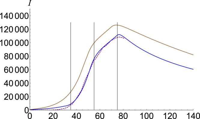
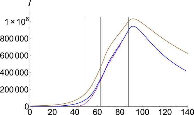
In Fig. 7, Fig. 8 we plot the infectious estimation for Italy [14] and the USA [15], respectively. Phases distribution together with basic reproduction numbers are given in Table 1.

Fig. 7.

Infected number $I$ for Italy. Data is plotted with purple, SEIR solution with brown, and the fractional model $c_1={\lambda }_1=0.9$, $c_2={\lambda }_2=1.25$, $c_3={\lambda }_3=1.3$, $c_4={\lambda }_4=1.1$ and $b_4={\eta }_4=1.25$ with blue.(For interpretation of the references to color in this figure legend, the reader is referred to the web version of this article.)

Fig. 8.

Infected number $I$ for USA. Data is plotted with purple, SEIR solution with brown, and the fractional model $c_1={\lambda }_1=0.9$, $c_2={\lambda }_2=1.15$, $c_3={\lambda }_3=1.2$, $c_4={\lambda }_4=1$ and $b_4={\eta }_4=1.15$ with blue.(For interpretation of the references to color in this figure legend, the reader is referred to the web version of this article.)

Conclusions

In this paper, after introducing elementary notions regarding fractional calculus, we calculate the generalized fractional-order Bernoulli polynomials, necessary to develop our numerical method. Although the correctness of the model depends on the already known information, we can adjust this inconvenience by fitting the model to the real-world data using fractional coefficients and therefore to better predict the near future. We learned from China that the fractional calculus improves the infection estimation by several thousand cases. Therefore, it is necessary to investigate the complex dynamical behaviors, especially chaos, in a such complex system how is an epidemic. Checking our model on the already existing data of the epidemic in Wuhan, China and South Korea we use it for better predict the epidemic in Italy and the USA.

The later stages of the epidemic are highly dependent on the influence of the number of infections in the first stage. According to the analysis of the dynamics of the proposed model, the best way to protect people from Covid-19 is to limit the interaction between health workers treating the infected, as they are more likely to become infected themselves, and to infect the general population. Our results are in accordance with the conditions required by [11] such as wearing a mask and keeping the social distance.

References

- 1.Chen S., Chang C., Liao C. Predictive models of control strategies involved in containing indoor airborne infections. Indoor Air. 2006;16(6):469–481. doi: 10.1111/j.1600-0668.2006.00443.x. [DOI] [PubMed] [Google Scholar]
- 2.Chen N., Zhou M., Dong X., Qu J., Gong F., Han Y., Qiu Y., Wang J., Liu Y., Wei Y. Epidemiological and clinical characteristics of 99 cases of 2019 novel coronavirus pneumonia in Wuhan, China: a descriptive study. Lancet. 2020;395(10223):507–513. doi: 10.1016/S0140-6736(20)30211-7. [DOI] [PMC free article] [PubMed] [Google Scholar]
- 3.Chowell G., Hengartner N.W., Castillo-Chavez C., Fenimore P.W., Hyman J.M. The basic reproductive number of Ebola and the effects of public health measures: the cases of Congo and Uganda. J. Theoret. Biol. 2004;229(1):119–126. doi: 10.1016/j.jtbi.2004.03.006. [DOI] [PubMed] [Google Scholar]
- 4.Chowell G., Nishiura H., Bettencourt L.M. Comparative estimation of the reproduction number for pandemic influenza from daily case notification data. J. R. Soc. Interface. 2007;4(12):155–166. doi: 10.1098/rsif.2006.0161. [DOI] [PMC free article] [PubMed] [Google Scholar]
- 5.Fang H., Chen J., Hu J. 2005 IEEE Engineering in Medicine and Biology 27th Annual Conference. IEEE; 2006. Modelling the SARS epidemic by a lattice-based Monte-Carlo simulation; pp. 7470–7473. [DOI] [PubMed] [Google Scholar]
- 6.Fang Z., Thieme H.R. Recurrent outbreaks of childhood diseases revisited: the impact of isolation. Math. Biosci. 1995;128(1–2):93–130. doi: 10.1016/0025-5564(94)00069-c. [DOI] [PubMed] [Google Scholar]
- 7.Feng Z., Yang Y., Xu D., Zhang P., McCauley M.M., Glasser J.W. Timely identification of optimal control strategies for emerging infectious diseases. J. Theoret. Biol. 2009;259(1):165–171. doi: 10.1016/j.jtbi.2009.03.006. [DOI] [PMC free article] [PubMed] [Google Scholar]
- 8.Getz W.M., Salter R., Mgbara W. Adequacy of SEIR models when epidemics have spatial structure: Ebola in Sierra Leone. Phil. Trans. R. Soc. B. 2019;374(1775) doi: 10.1098/rstb.2018.0282. [DOI] [PMC free article] [PubMed] [Google Scholar]
- 9.Hartley T.T., Lorenzo C.F., Qammer H.K. Chaos in a fractional order Chua’s system. IEEE Trans. Circuits Syst. I. 1995;42(8):485–490. [Google Scholar]
- 10.https://www.bsg.ox.ac.uk/research/research-projects/coronavirus-government-response-tracker.
- 11.https://www.cdc.gov/coronavirus/2019-ncov/prevent-getting-sick/prevention.html.
- 12.https://www.worldometers.info/coronavirus/country/china/.
- 13.https://www.worldometers.info/coronavirus/country/south-korea/.
- 14.https://www.worldometers.info/coronavirus/country/italy/.
- 15.https://www.worldometers.info/coronavirus/country/us/.
- 16.Hyman J.M., Li J. Modeling the effectiveness of isolation strategies in preventing STD epidemics. SIAM J. Appl. Math. 1998;58(3):912–925. [Google Scholar]
- 17.Kar T., Batabyal A. Modeling and analysis of an epidemic model with non-monotonic incidence rate under treatment. J. Math. Res. 2010;2(1):103. [Google Scholar]
- 18.Kumar D., Singh J., Al Qurashi M., Baleanu D. A new fractional SIRS-SI malaria disease model with application of vaccines, antimalarial drugs, and spraying. Adv. Difference Equ. 2019;2019(1):278. [Google Scholar]
- 19.Li J., Cui N. Dynamic analysis of an SEIR model with distinct incidence for exposed and infectives. Sci. World J. 2013;2013 doi: 10.1155/2013/871393. [DOI] [PMC free article] [PubMed] [Google Scholar]
- 20.Liu N., Fang J., Deng W., Sun J.-w. Stability analysis of a fractional-order SIS model on complex networks with linear treatment function. Adv. Difference Equ. 2019;2019(1):1–10. [Google Scholar]
- 21.Liu W., Fontanet A., Zhang P.-H., Zhan L., Xin Z.-T., Baril L., Tang F., Lv H., Cao W.-C. Two-year prospective study of the humoral immune response of patients with severe acute respiratory syndrome. J. Infec. Dis. 2006;193(6):792–795. doi: 10.1086/500469. [DOI] [PMC free article] [PubMed] [Google Scholar]
- 22.Odibat Z.M., Shawagfeh N.T. Generalized Taylor’s formula. Appl. Math. Comput. 2007;186(1):286–293. [Google Scholar]
- 23.Peak C.M., Childs L.M., Grad Y.H., Buckee C.O. Comparing nonpharmaceutical interventions for containing emerging epidemics. Proc. Natl. Acad. Sci. 2017;114(15):4023–4028. doi: 10.1073/pnas.1616438114. [DOI] [PMC free article] [PubMed] [Google Scholar]
- 24.Podlubny I. Elsevier; 1998. Fractional Differential Equations: an Introduction to Fractional Derivatives, Fractional Differential Equations, to Methods of Their Solution and Some of Their Applications. [Google Scholar]
- 25.Rachah A. Analysis, simulation and optimal control of a SEIR model for Ebola virus with demographic effects. Commun. Fac. Sci. Univ. Ankara Ser. A1 Math. Stat. 2018;67(1):179–197. [Google Scholar]
- 26.ur Rehman M., Khan R.A. A numerical method for solving boundary value problems for fractional differential equations. Appl. Math. Model. 2012;36(3):894–907. [Google Scholar]
- 27.Rihan F., Al-Mdallal Q., AlSakaji H., Hashish A. A fractional-order epidemic model with time-delay and nonlinear incidence rate. Chaos Solitons Fractals. 2019;126:97–105. [Google Scholar]
- 28.Saito M.M., Imoto S., Yamaguchi R., Sato H., Nakada H., Kami M., Miyano S., Higuchi T. Extension and verification of the SEIR model on the 2009 influenza a (H1N1) pandemic in Japan. Math. Biosci. 2013;246(1):47–54. doi: 10.1016/j.mbs.2013.08.009. [DOI] [PubMed] [Google Scholar]
- 29.Shu H., Fan D., Wei J. Global stability of multi-group SEIR epidemic models with distributed delays and nonlinear transmission. Nonlinear Anal. RWA. 2012;13(4):1581–1592. [Google Scholar]
- 30.Smirnova A., deCamp L., Chowell G. Forecasting epidemics through nonparametric estimation of time-dependent transmission rates using the SEIR model. Bull. Math. Biol. 2019;81(11):4343–4365. doi: 10.1007/s11538-017-0284-3. [DOI] [PubMed] [Google Scholar]
- 31.Sun C., Hsieh Y.-H. Global analysis of an SEIR model with varying population size and vaccination. Appl. Math. Model. 2010;34(10):2685–2697. [Google Scholar]
- 32.Tri Putra R. Kestabilan lokal bebas penyakit model epidemi seir dengan kemampuan infeksi pada periode laten, infeksi dan sembuh. Rekayasa Sipil. 2011;7(1):42–52. [Google Scholar]
- 33.Wang D., Hu B., Hu C., Zhu F., Liu X., Zhang J., Wang B., Xiang H., Cheng Z., Xiong Y. Clinical characteristics of 138 hospitalized patients with 2019 novel coronavirus–infected pneumonia in Wuhan, China. JAMA. 2020;323(11):1061–1069. doi: 10.1001/jama.2020.1585. [DOI] [PMC free article] [PubMed] [Google Scholar]
- 34.Wang J., Liu S., Zheng B., Takeuchi Y. Qualitative and bifurcation analysis using an SIR model with a saturated treatment function. Math. Comput. Model. 2012;55(3–4):710–722. [Google Scholar]
- 35.Wendi W. Backward bifurcation of an epidemic model with treatment. Math. Biosci. 2006;201(1–2):58–71. doi: 10.1016/j.mbs.2005.12.022. [DOI] [PubMed] [Google Scholar]
- 36.Wu L.-I., Feng Z. Homoclinic bifurcation in an SIQR model for childhood diseases. J. Differential Equations. 2000;168(1):150–167. [Google Scholar]
- 37.Yi N., Zhang Q., Mao K., Yang D., Li Q. Analysis and control of an SEIR epidemic system with nonlinear transmission rate. Math. Comput. Model. 2009;50(9–10):1498–1513. doi: 10.1016/j.mcm.2009.07.014. [DOI] [PMC free article] [PubMed] [Google Scholar]
- 38.YüZbaşı Ş., ŞAhin N., Sezer M. Numerical solutions of systems of linear Fredholm integro-differential equations with Bessel polynomial bases. Comput. Math. Appl. 2011;61(10):3079–3096. [Google Scholar]
- 39.Zhang J., Li J., Ma Z. Global dynamics of an SEIR epidemic model with immigration of different compartments. Acta Math. Sci. 2006;26(3):551–567. [Google Scholar]
- 40.Zhang X., Liu X. Backward bifurcation of an epidemic model with saturated treatment function. J. Math. Anal. Appl. 2008;348(1):433–443. [Google Scholar]
- 41.Zhou X., Cui J. Analysis of stability and bifurcation for an SEIR epidemic model with saturated recovery rate. Commun. Nonlinear Sci. Numer. Simul. 2011;16(11):4438–4450. [Google Scholar]