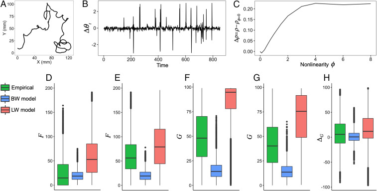
Fig. 5.

Empirical analysis. (A and B) Example of a movement trajectory of Drosophila larvae and the corresponding time series of turning angles, respectively. (C) Example of the result of S-map to check nonlinearity of the time series. (D–H) The results of perturbation analysis. (D and E) The corresponding cases of small and large $S$ for $\tau =100$, respectively. (F and G) The corresponding cases of small and large $S^{\prime }$ for $\tau =100$, respectively. (H) The difference of $G$ between F and G. Note that BW and LW model mean the proposed model with $\epsilon =0.0$ and 0.22, respectively. In D–H, all pairwise differences among the empirical, BW model, and LW model were statistically significant ($p<10^{-15}$). The black dots in D–H represent outliers, defined as data points outside the whiskers, which correspond to 1.5 times the interquartile range.