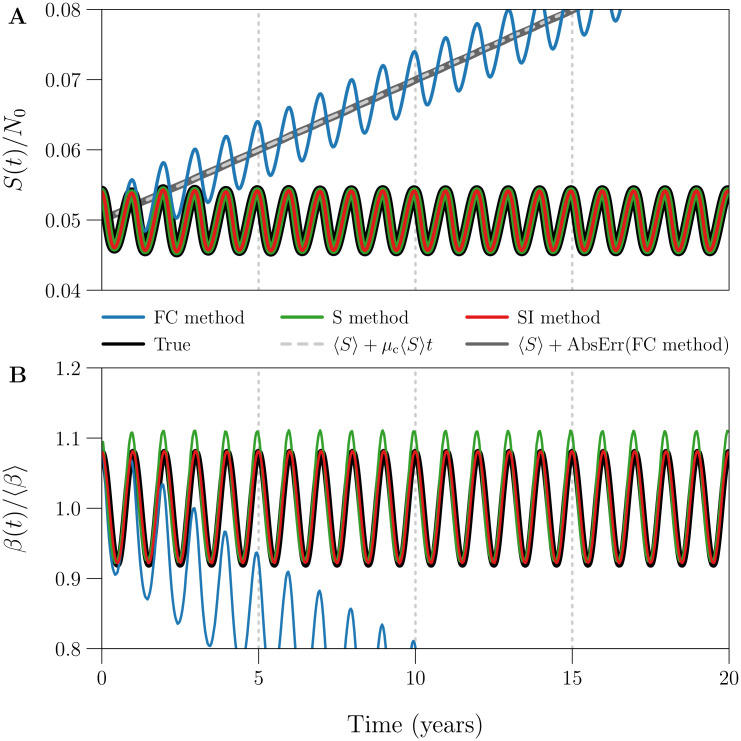
Fig 1. Example of S(t) and β(t) estimation using the FC, S, and SI methods.

Plotted are the susceptible population size S(t) and seasonally forced transmission rate β(t) (Eq (27)) underlying 20 years of weekly reported incidence, together with time series estimates S_k and β_k obtained from the data by the FC [blue], S [green], and SI [red] methods. The reported incidence time series (Δt = 1 week, n = ⌊20 × 365/7⌋ = 1042) was simulated without process or observation error (ϵ = 0, p_rep = 1), using reference values (Table 1) for all other data-generating parameters. The three estimation methods were applied without input error, i.e., all input parameters were assigned their true (data-generating) values. [Panel A] S(t) scaled by 1/N₀, describing the number of susceptibles as a proportion of the initial population size. Grey lines show that the absolute error in the FC method estimate of S(t) increases linearly as μ_c 〈S〉t, where μ_c is the constant per capita natural mortality rate and 〈S〉 is the continuous-time average of S(t). [Panel B] β(t) scaled by 1/〈β〉, describing the transmission rate relative to its mean. RRMSE (Eq (33)) in the β_k time series generated by the (FC, S, SI) method is roughly (0.3355, 0.0240, 0.0021).