A Mathematical Model to Investigate the Transmission of COVID-19 in the Kingdom of Saudi Arabia

Abstract

Since the first confirmed case of SARS-CoV-2 coronavirus (COVID-19) on March 02, 2020, Saudi Arabia has not reported quite a rapid COVD-19 spread as seen in America and many European countries. Possible causes include the spread of asymptomatic COVID-19 cases. To characterize the transmission of COVID-19 in Saudi Arabia, a susceptible, exposed, symptomatic, asymptomatic, hospitalized, and recovered dynamical model was formulated, and a basic analysis of the model is presented including model positivity, boundedness, and stability around the disease-free equilibrium. It is found that the model is locally and globally stable around the disease-free equilibrium when R₀ < 1. The model parameterized from COVID-19 confirmed cases reported by the Ministry of Health in Saudi Arabia (MOH) from March 02 till April 14, while some parameters are estimated from the literature. The numerical simulation showed that the model predicted infected curve is in good agreement with the real data of COVID-19-infected cases. An analytical expression of the basic reproduction number R₀ is obtained, and the numerical value is estimated as R₀ ≈ 2.7.

1. Introduction

As of April 22, 2020, more than 12772 cases and 114 deaths of coronavirus disease 2019 (COVID-19) caused by the SARS-CoV-2 virus had been confirmed in the Kingdom of Saudi Arabia. Since March 04 [1], control measures have been implemented within Saudi Arabia to control the spread of the disease. Isolation of confirmed cases and contact tracing are crucial parts of these measures, which are common interventions for controlling infectious disease outbreaks [2–4]. For example, the severe acute respiratory syndrome (SARS) outbreak and the Middle East respiratory syndrome (MERS) were controlled through tracing suspected cases and isolating confirmed cases because the majority of transmission occurred concurrent or after symptom onset [3–5].

However, it is unknown if transmission of COVID-19 can occur before symptom onset, which could decrease the effectiveness of isolation and contact tracing [2, 3, 5].

In this paper, the impact of asymptomatic COVID-19 cases on the spread of the disease is considered using a modified version of the susceptible-exposed-infected-recovered (SEIR) dynamical model, along with the data of COVID-19 cases reported daily by the Ministry of Health in Saudi Arabia (MOH). Other main objectives of this paper include obtaining an analytical expression and numerical estimation of the basic reproduction number R₀ of COVID-19 in Saudi Arabia and estimating the maximum required number of hospital beds and intensive care units (ICU). The rest of this study is organized as follows: The model establishment is presented in Section 2. Basic analysis of the model, including local and global stability results of the disease-free equilibrium, is explored in Section 3. The model fitting to daily reported cases and estimation of parameters is given in Section 4. Numerical results and discussion are presented in Section 5. Finally, brief concluding remarks are given in Section 6.

2. Model Establishment

The Saudi population Q will be divided into six categories: susceptible (S), exposed (E), symptomatic (Y), asymptomatic (N), hospitalized (H), and recovered (R) individuals (SEYNHR). Individuals move from the susceptible compartment S to the exposed compartment E after interacting with infected individuals with transmission rates β₁, β₂, and β₃ as shown in Figure 1. COVID-19 is known to have an incubation period, from 2 to 14 days, between exposure and development of symptoms [6, 7]. After this period, exposed individual transits from the compartment E to either compartment Y at a rate α or compartment N at a rate α(1 − γ). An individual could move from compartment N to Y at a rate K if they show symptoms. Once an individual becomes infected with the coronavirus that causes COVID-19, that individual develops immunity against the virus with a rate Φ_Y or the individual will be hospitalized with a rate of ε or dies because of the disease with a rate of μ₁. When an individual becomes hospitalized, that individual receives treatment and develops immunity against the virus with a rate r or dies because of the disease with a rate μ₂.

Figure 1.

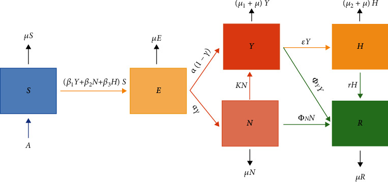
Schematic diagram of the SEYNHR compartment model. The arrows, except the black ones, represent a progression from one compartment to the next.

As shown in Figure 1, the SEYNHR model has six compartments; therefore, a discrete dynamical system consisting of six nonlinear differential equations is formed as follows:

$$\begin{array}{c}\frac{dS}{dt}=A-\left({\beta }_{1}Y+{\beta }_{2}N+{\beta }_{3}H\right)S-\mu S,\end{array}$$ (1)

$$\begin{array}{c}\frac{dE}{dt}=\left({\beta }_{1}Y+{\beta }_{2}N+{\beta }_{3}H\right)S-\left(\alpha +\mu \right)E,\end{array}$$ (2)

$$\begin{array}{c}\frac{dY}{dt}=\alpha \left(1-\gamma \right)E-\left({\mathrm{\Phi }}_Y+\epsilon +{\mu }_1+\mu \right)Y+KN,\end{array}$$ (3)

$$\begin{array}{c}\frac{dN}{dt}=\alpha \gamma E-\left({\mathrm{\Phi }}_N+K+\mu \right)N,\end{array}$$ (4)

$$\begin{array}{c}\frac{dH}{dt}=\epsilon Y-\left(r+{\mu }_2+\mu \right)H,\end{array}$$ (5)

$$\begin{array}{c}\frac{dR}{dt}={\mathrm{\Phi }}_{Y}Y+{\mathrm{\Phi }}_{N}N+rH-\mu R,\end{array}$$ (6)

where Q(t) = S(t) + E(t) + Y(t) + N(t) + H(t) + R(t) and Q(t) is the Saudi population at time t. The next-generation matrix is used in the next section to derive an analytical expression of the basic reproduction number R₀, for the compartmental model above. Calculating R₀ is a useful metric for assessing the transmission potential of an emerging COVID-19 in Saudi Arabia.

3. Basic Analytical Results

In this section, the positivity and boundedness of the proposed SEYNHR model solution (6) and stability of the model around the disease-free equilibrium is investigated. Furthermore, an analytical expression of the basic reproduction number R₀ is established.

3.1. Positivity and Boundedness

To show that the SEYNHR model (6) is biologically well-behaved or epidemiologically meaningful, we must show that all its state variables are nonnegative and bounded for t > 0.

$$\begin{array}{c}\frac{dS}{dt}=A-\left({\beta }_{1}Y\left(t\right)+{\beta }_{2}N\left(t\right)+{\beta }_{3}H\left(t\right)\right)S\left(t\right)-\mu S\left(t\right).\end{array}$$ (7)

Lemma 1 . —

For t > 0 and initial values P(0) ≥ 0, where P(t) = (S(t), E(t), Y(t), N(t), H(t), R(t)), the solution of the SEYNHR model (6) is nonnegative if they exist.

Proof —

Assume t₁ = {t > 0 : P(t) > 0 ∈ [0, t]}, then it follows from the first equation of (6) as

It can be written as

$$\begin{array}{c}\frac{dS}{dt}\left\{S\left(t\right)\exp \left(\mu t+{\int }_0^t\left({\beta }_{1}Y\left(\zeta \right)+{\beta }_{2}N\left(\zeta \right)+{\beta }_{3}H\left(\zeta \right)\right)S\left(\zeta \right)d\zeta \right)\right\}-A\exp \left(\mu t+{\int }_0^t\left({\beta }_{1}Y\left(\zeta \right)+{\beta }_{2}N\left(\zeta \right)+{\beta }_{3}H\left(\zeta \right)\right)S\left(\zeta \right)d\zeta \right)=0.\end{array}$$ (8)

Hence,

$$\begin{array}{c}S\left(t_1\right)\exp \left(\mu t_1+{\int }_0^{t_1}\left({\beta }_{1}Y\left(\zeta \right)+{\beta }_{2}N\left(\zeta \right)+{\beta }_{3}H\left(\zeta \right)\right)S\left(\zeta \right)d\zeta \right)-S\left(0\right)={\int }_0^{t_1}A\exp \left(\mu p+{\int }_0^p\left({\beta }_{1}Y\left(\zeta \right)+{\beta }_{2}N\left(\zeta \right)+{\beta }_{3}H\left(\zeta \right)\right)S\left(\zeta \right)d\zeta \right)dp,\end{array}$$ (9)

which can be found as below

$$\begin{array}{c}S\left(t_1\right)=S\left(0\right)\exp \left\{-\left(\mu t_1+{\int }_0^{t_1}\left({\beta }_{1}Y\left(\zeta \right)+{\beta }_{2}N\left(\zeta \right)+{\beta }_{3}H\left(\zeta \right)\right)S\left(\zeta \right)d\zeta \right)\right\}+\exp \left\{-\left(\mu t_1+{\int }_0^{t_1}\left({\beta }_{1}Y\left(\zeta \right)+{\beta }_{2}N\left(\zeta \right)+{\beta }_{3}H\left(\zeta \right)\right)S\left(\zeta \right)d\zeta \right)\right\}\times {\int }_0^{t_1}A\exp \left(\mu p+{\int }_0^p\left({\beta }_{1}Y\left(\zeta \right)+{\beta }_{2}N\left(\zeta \right)+{\beta }_{3}H\left(\zeta \right)\right)S\left(\zeta \right)d\zeta \right)dp>0.\end{array}$$ (10)

Hence, S(t) is nonnegative for t > 0. In a similar way, it can be shown that E > 0, Y > 0, N > 0, H > 0, and R > 0 for t > 0.

$$\begin{array}{c}\frac{dQ}{dt}=A-\mu Q\left(t\right)-{\mu }_{1}Y-{\mu }_{2}H\le A-\mu Q\left(t\right).\end{array}$$ (11)

Lemma 2 . —

Ω = {(S(t), E(t), Y(t), N(t), H(t), R(t)) ∈ R₊⁶ ∪ {0}: 0 < S(t) + E(t) + Y(t) + N(t) + H(t) + R(t) ≤ A/μ} is the positively invariant region of the model (6) with nonnegative initial conditions in R₊⁶.

Proof —

Suppose Q(t) = S(t) + E(t) + Y(t) + N(t) + H(t) + R(t) holds for t ≥ 0, then we get

It is obvious that

$$\begin{array}{c}Q\left(t\right)\le Q\left(0\right)e^{-\mu t}+\frac{A}{\mu }\left(1-e^{-\mu t}\right).\end{array}$$ (12)

Thus, lim_t⟶∞sup Q(t) ≤ A/μ. Furthermore, (dQ(t))/dt < 0 if Q(t) > A/μ. This shows that solutions of the model (6) point towards Ω. Hence, Ω is positively invariant and solutions of (6) are bounded.

3.2. Basic Reproduction Number R₀

It can be easily verified that system (6) always has a disease-free equilibrium (DFE), which we will denote by E₀, and it is given by

$$\begin{array}{c}{E}_0=\left(\frac{A}{\mu },0,0,0,0,0\right).\end{array}$$ (13)

Next, we investigate an important concept in epidemiology which is the basic reproduction number, defined as “the expected number of secondary cases produced, in a completely susceptible population, by a typical infective individual” [8]. The next-generation method is used to calculate R₀; more details about the method are in [8]. The system (6) can be rewritten as follows:

$$\begin{array}{c}\frac{dw}{dt}=\mathrm{\Phi }\left(w\right)-\mathrm{\Psi }\left(w\right),\end{array}$$ (14)

where F≔(F1, F2, F3, F4, F5, F6)^T and V≔(V1, V2, V3, V4, V5, V6)^T, or more explicitly

$$\begin{array}{c}\left(\begin{array}{c}\dot{E}\\ \dot{Y}\\ \dot{N}\\ \dot{H}\\ \dot{R}\\ \dot{S}\end{array}\right)=\left(\begin{array}{c}\left({\beta }_{1}Y+{\beta }_{2}N+{\beta }_{3}H\right)S\\ 0\\ 0\\ 0\\ 0\\ 0\end{array}\right)-\left(\begin{array}{c}\left(\alpha +\mu \right)E\\ \left({}_Y+\epsilon +{\mu }_1+\mu \right)Y-\alpha \left(1-\gamma \right)\ast E-KN\\ \left({\mathrm{\Phi }}_N+K+\mu \right)N-\alpha \gamma E\\ \left(r+{\mu }_2+\mu \right)H-\epsilon Y\\ \left(P+\mu \right)R-{\mathrm{\Phi }}_Y-{\mathrm{\Phi }}_N-rH\\ \left({\beta }_{1}Y+{\beta }_{2}N+{\beta }_{3}H\right)S-A-PR\end{array}\right).\end{array}$$ (15)

The Jacobian matrices of F and V evaluated at the solution E₀^∗ = (0, 0, 0, 0, 0, A/μ)^T are given by

$$\begin{array}{c}{\left.F=\left({\frac{\partial {\mathrm{\Phi }}_i}{\partial w_j}}_{E_0^{\ast }}\right)\right|}_{\begin{array}{c}1\le i,j\le 4\end{array}}=\left(\begin{array}{cccc}0& \frac{{\beta }_{1}A}{\mu }& \frac{{\beta }_{2}A}{\mu }& \frac{{\beta }_{3}A}{\mu }\\ 0& 0& 0& 0\\ 0& 0& 0& 0\\ 0& 0& 0& 0\end{array}\right),\\ {\left.V=\left({\frac{\partial {\mathrm{\Psi }}_i}{\partial w_j}}_{\begin{array}{c}{E}_0^{\ast }\end{array}}\right)\right|}_{\begin{array}{c}1\le i,j\le 4\end{array}}=\left(\begin{array}{cccc}\alpha +\mu & 0& 0& 0\\ -\alpha \left(1-\gamma \right)& {\mathrm{\Phi }}_Y+\epsilon +{\mu }_1+\mu & -K& 0\\ -\alpha \gamma & 0& {\mathrm{\Phi }}_N+K+\mu & 0\\ 0& -\epsilon & 0& r+{\mu }_2+\mu \end{array}\right).\end{array}$$ (16)

Direct calculations show that

$$\begin{array}{c}{V}^{-1}=\left(\begin{array}{cccc}\frac{1}{\alpha +\mu }& 0& 0& 0\\ m_1& m_4& m_6& 0\\ m_2& 0& m_7& 0\\ m_3& m_5& m_8& \frac{1}{r+{\mu }_2+\mu }\end{array}\right),\end{array}$$ (17)

where

$$\begin{array}{c}\left\{\begin{array}{cc}{m}_1=\hfill & \frac{\alpha \left(1-\gamma \right)K+\alpha \left(1-\gamma \right)\mu +\alpha \left(1-\gamma \right){\mathrm{\Phi }}_N+K\alpha \gamma }{\left({\mathrm{\Phi }}_Y+\epsilon +{\mu }_1+\mu \right)\left({\mathrm{\Phi }}_N+K+\mu \right)\left(\alpha +\mu \right)},\hfill \\ \hfill & \hfill \\ m_2=\hfill & \frac{\alpha \gamma }{\left(\alpha +\mu \right)\left({\mathrm{\Phi }}_N+K+\mu \right)},\hfill \\ m_3=\hfill & \frac{\epsilon \left(\alpha \left(1-\gamma \right)K+\alpha \left(1-\gamma \right)\mu +\alpha \left(1-\gamma \right){\mathrm{\Phi }}_N+K\alpha \gamma \right)}{\left({\mathrm{\Phi }}_Y+\epsilon +{\mu }_1+\mu \right)\left({\mathrm{\Phi }}_N+K+\mu \right)\left(\alpha +\mu \right)\left(r+{\mu }_2+\mu \right)},\hfill \\ m_4=\hfill & \frac{1}{{\mathrm{\Phi }}_Y+\epsilon +{\mu }_1+\mu },\hfill \\ m_5=\hfill & \frac{\epsilon }{\left({\mathrm{\Phi }}_Y+\epsilon +{\mu }_1+\mu \right)\left(r+{\mu }_2+\mu \right)},\hfill \\ m_6=\hfill & \frac{K}{\left({\mathrm{\Phi }}_N+K+\mu \right)\left({\mathrm{\Phi }}_Y+\epsilon +{\mu }_1+\mu \right)},\hfill \\ m_7=\hfill & \frac{1}{{\mathrm{\Phi }}_N+K+\mu },\hfill \\ m_8=\hfill & \frac{\epsilon K}{\left({\mathrm{\Phi }}_Y+\epsilon +{\mu }_1+\mu \right)\left({\mathrm{\Phi }}_N+K+\mu \right)\left(r+{\mu }_2+\mu \right)}.\hfill \\ \hfill & \hfill \end{array}\right.\end{array}$$ (18)

Denoting the 4 × 4 identity matrix by ℐ, the characteristic polynomial Γ(λ) of the matrix FV⁻¹ is given by

$$\begin{array}{c}\begin{array}{cc}\mathrm{\Gamma }\left(\lambda \right)& =\det \left(F{V}^{-1}-\lambda \mathcal{I}\right),\\ & =\frac{-{\lambda }^3\left(\left({\mathrm{\Phi }}_N+K+\mu \right)\left({\beta }_1\mu +\left(r+{\mu }_2\right){\beta }_1+{\beta }_3\epsilon \right)A\alpha \left(1-\gamma \right)+\left(B_1+B_2\right)A\alpha \gamma \right)+{\lambda }^4}{\mu \left({\mathrm{\Phi }}_Y+\epsilon +{\mu }_1+\mu \right)\left({\mathrm{\Phi }}_N+K+\mu \right)\left(\alpha +\mu \right)\left(r+{\mu }_2+\mu \right)},\\ & \end{array}\end{array}$$ (19)

where

$$\begin{array}{c}\left\{\begin{array}{c}{B}_1={\beta }_2{\mu }^2+\left(\left({\mu }_1+{\mu }_2+{\mathrm{\Phi }}_Y+\epsilon +r\right){\beta }_2+{\beta }_{1}K\right)\mu +K\left(r+{\mu }_2\right){\beta }_1,\hfill \\ B_2=\left(r+{\mu }_2\right)\left({\mathrm{\Phi }}_Y+\epsilon +{\mu }_1\right){\beta }_2+{\beta }_3\epsilon K.\hfill \end{array}\right.\end{array}$$ (20)

The solutions λ_1,2,3,4 are given by

$$\begin{array}{c}\left\{0,0,0,\frac{\left({\mathrm{\Phi }}_N+K+\mu \right)\left({\beta }_1\mu +\left(r+{\mu }_2\right){\beta }_1+{\beta }_3\epsilon \right)A\alpha \left(1-\gamma \right)+\left(B_1+B_2\right)A\alpha \gamma }{\mu \left({\mathrm{\Phi }}_Y+\epsilon +{\mu }_1+\mu \right)\left({\mathrm{\Phi }}_N+K+\mu \right)\left(\alpha +\mu \right)\left(r+{\mu }_2+\mu \right)}\right\}.\end{array}$$ (21)

Therefore, the reproduction number R₀ for the SEYNHR model (6) is given by

$$\begin{array}{c}{R}_0=\max \left\{{\lambda }_1,{\lambda }_2,{\lambda }_3,{\lambda }_4\right\},=\frac{\left({\mathrm{\Phi }}_N+K+\mu \right)\left({\beta }_1\mu +\left(r+{\mu }_2\right){\beta }_1+{\beta }_3\epsilon \right)A\alpha \left(1-\gamma \right)+\left(B_1+B_2\right)A\alpha \gamma }{\mu \left({\mathrm{\Phi }}_Y+\epsilon +{\mu }_1+\mu \right)\left({\mathrm{\Phi }}_N+K+\mu \right)\left(\alpha +\mu \right)\left(r+{\mu }_2+\mu \right)}.\end{array}$$ (22)

For simplicity, let us denote

$$\begin{array}{c}{\rho }_1=\alpha +\mu ,\\ {\rho }_2={\mathrm{\Phi }}_Y+\epsilon +{\mu }_1+\mu ,\\ {\rho }_3={\mathrm{\Phi }}_N+K+\mu ,\\ {\rho }_4=r+{\mu }_2+\mu .\end{array}$$ (23)

In order to interpret the basic reproduction number R₀, we split the above expression of R₀ as follows:

$$\begin{array}{c}{R}_0=R_{YH}+R_{EYNH1}+R_{EYNH2},\end{array}$$ (24)

where

$$\begin{array}{c}{R}_{YH}=\alpha \left(1-\gamma \right)\times \frac{A}{\mu }\times \frac{1}{{\rho }_1}\times \frac{1}{{\rho }_1{\rho }_4}\times \left({\beta }_1{\rho }_4+{\beta }_3\epsilon \right),\\ R_{EYNH1}=\alpha \gamma \times \frac{A}{\mu }\times \left(\frac{1}{{\rho }_1{\rho }_2{\rho }_3{\rho }_4}\times {\beta }_3{\mu }^2\frac{1}{{\rho }_1{\rho }_2{\rho }_3{\rho }_4}\times {\beta }_{1}K\left(r+{\mu }_2\right)+\frac{1}{{\rho }_1{\rho }_2{\rho }_3{\rho }_4}\times \left(\left({\mu }_1+{\mu }_2+{\mathrm{\Phi }}_Y+\epsilon +r\right){\beta }_2+{\beta }_{1}K\right)\mu \right),\\ R_{EYNH2}=\alpha \gamma \times \frac{A}{\mu }\left(\frac{1}{{\rho }_1{\rho }_2{\rho }_3{\rho }_4}\times {\beta }_2\left(r+{\mu }_2\right)\left({\rho }_2-\mu \right)+\frac{1}{{\rho }_1{\rho }_2{\rho }_3{\rho }_4}\times {\beta }_1\epsilon K\right).\end{array}$$ (25)

The first and second terms in R_YH show the probability of the total population becoming symptomatic upon infection multiplied by mean symptomatic, exposed, and hospitalized infectious periods multiplied by symptomatic and hospitalized contact rates. The first and second terms in R_EYNH1 show the probability of the total population becoming asymptomatic multiplied by mean exposed, symptomatic, asymptomatic, and hospitalized infectious periods multiplied by symptomatic, asymptomatic, and hospitalized contact rates. Furthermore, the first and second terms in R_EYNH2 show the probability of the total population becoming asymptomatic multiplied by mean exposed, symptomatic, asymptomatic, and hospitalized infectious periods multiplied by asymptomatic and hospitalized contact rates. The obtained analytical expression of R₀ shows that asymptomatic as well as symptomatic cases of COVID-19 could drive the growth of the pandemic in Saudi Arabia.

3.3. Stability of Disease-Free Equilibrium

In this section, the local and global stability of the model (6) around the disease-free equilibrium is explored. The epidemiological implication of the local stability result of DFE is that a small influx of COVID-19 infection cases will not generate a COVID-19 outbreak if R₀ < 1 while the global stability result of DFE indicates that any influx of COVID-19 infection cases will not generate a COVID-19 outbreak if R₀ < 1.

$$\begin{array}{c}{J}_{E_0}=\left(\begin{array}{cccccc}-\mu & 0& -\frac{{\beta }_{1}A}{\mu }& -\frac{{\beta }_{2}A}{\mu }& -\frac{{\beta }_{3}A}{\mu }& 0\\ 0& -\left(\alpha +\mu \right)& \frac{{\beta }_{1}A}{\mu }& \frac{{\beta }_{2}A}{\mu }& \frac{{\beta }_{3}A}{\mu }& 0\\ 0& \alpha \left(1-\gamma \right)& -\left({\mathrm{\Phi }}_Y+\epsilon +{\mu }_1+\mu \right)& K& 0& 0\\ 0& \alpha \gamma & 0& -\left({\mathrm{\Phi }}_N+K+\mu \right)& 0& 0\\ 0& 0& \epsilon & 0& -\left(r+{\mu }_2+\mu \right)& 0\\ 0& 0& {\mathrm{\Phi }}_Y& {\mathrm{\Phi }}_N& r& -\mu \end{array}\right).\end{array}$$ (26)

Theorem 1 . —

The DFE E₀ of the system (6) is locally asymptotically stable if R₀ < 1 and unstable otherwise.

Proof —

The Jacobian matrix J_E0 obtained at the DFE E₀ is as follows:

Clearly, the eigenvalues −μ and −μ are negative real numbers. The remaining eigenvalues can be obtained through the following equation:

$$\begin{array}{c}{\lambda }^4+C_1{\lambda }^3+C_2{\lambda }^2+C_3\lambda +C_4=0,\end{array}$$ (27)

where

$$\begin{array}{c}\left\{\begin{array}{cc}{C}_1=\hfill & {\mathrm{\Phi }}_Y+{\mathrm{\Phi }}_N+K+4\mu +\alpha +\epsilon +{\mu }_1+{\mu }_2+r,\hfill \\ C_2=\hfill & -\frac{A\alpha {\beta }_1\left(1-\gamma \right)}{\mu }+{\beta }_1{\rho }_1{\rho }_2{\rho }_3^2{\rho }_4\psi ,\hfill \\ C_3=\hfill & -\frac{\left(2A{\beta }_1\alpha +A\alpha \right)\left(1-\gamma \right)}{\mu }+{\rho }_1{\rho }_2{\rho }_3^2{\rho }_4\psi +2{\beta }_1{\rho }_1{\rho }_2{\rho }_3^2{\rho }_4\psi ,\hfill \\ C_4=\hfill & -\frac{\left(A{\beta }_1\alpha +A\alpha \right)\left(1-\gamma \right)}{\mu }+{\rho }_1{\rho }_2{\rho }_3^2{\rho }_4\psi +{\beta }_1{\rho }_1{\rho }_2{\rho }_3^2{\rho }_4\psi +\text{positive\hspace{0.17em}terms},\hfill \\ \hfill & \hfill \end{array}\right.\end{array}$$ (28)

where ψ = (β₁μ + (r + μ₂)β₁ + β₃ε) and C₁ is obviously positive. We can rewrite R₀ as

$$\begin{array}{c}{R}_0=\frac{A\alpha \left(1-\gamma \right)+\text{positive\hspace{0.17em}terms}}{\mu {\rho }_1{\rho }_2{\rho }_3^2{\rho }_4\psi }.\end{array}$$ (29)

Clearly if R₀ < 1, then C₂ is positive. Similarly, we can show that C₃ and C₄ are all positive if R₀ < 1. Further, it is easy to show the remaining Routh-Hurtwiz condition for the fourth-order polynomial (27). Thus, the DFE is locally asymptotically stable if R₀ < 1.

The global stability of DFE E₀ of the COVID-19 transmission model is studied in the following result.

$$\begin{array}{c}\Pi \left(t\right)=\frac{W_1}{Q}E+W_{2}Y+W_{3}N+W_{4}H,\end{array}$$ (30)

where W_i for i = 1, 2, 3, 4, are positive constants. Differentiating the function Π(t) with respect to t and using the solutions of system (6), we obtain

$$\begin{array}{c}\frac{\Pi \left(t\right)}{dt}=W_1\left[\frac{\left({\beta }_{1}Y+{\beta }_{2}N+{\beta }_{3}H\right)S}{Q}-\frac{{\rho }_{1}E}{Q}\right]+W_2\left[\alpha \left(1-\gamma \right)E-{\rho }_{2}Y+KY\right]+W_3\left[\alpha \gamma -{\rho }_{3}N\right]+W_4\left[\epsilon Y-{\rho }_{4}H\right]\le W_1\left[\left({\beta }_{1}Y+{\beta }_{2}N+{\beta }_{3}H\right)-{\rho }_{1}E\right]+W_2\left[\alpha \left(1-\gamma \right)E-{\rho }_{2}Y+KY\right]+W_3\left[\alpha \gamma -{\rho }_{3}N\right]+W_4\left[\epsilon Y-{\rho }_{4}H\right],\text{as\hspace{0.5em}}\frac{S+E}{Q}<1.=\left[W_2\alpha \left(1-\gamma \right)-{\rho }_1+W_3\alpha \gamma \right]E+\left[W_1{\beta }_1-W_2{\rho }_2+W_4\epsilon \right]Y+\left[W_1{\beta }_2-W_3{\rho }_3\right]N+\left[W_1{\beta }_3-W_4{\rho }_4\right]H={\rho }_1\left[\frac{W_2\alpha \left(1-\gamma \right)+W_3\alpha \gamma }{{\rho }_1}-1\right]E+\left[W_1{\beta }_1-W_2{\rho }_2+W_4\epsilon \right]Y{\rho }_1\left[\frac{W_2\alpha \left(1-\gamma \right)+W_3\alpha \gamma }{{\rho }_1}-1\right]E+\left[W_1{\beta }_1-W_2{\rho }_2+W_4\epsilon \right]Y+\left[W_1{\beta }_2-W_3{\rho }_3\right]N+\left[W_1{\beta }_3-W_4{\rho }_4\right]H\end{array}$$ (31)

Theorem 2 . —

The DFE E₀ of the system (6) is globally asymptotically stable if R₀ < 1 and unstable otherwise.

Proof —

Let us consider the following Lyapunov function, described in [9]:

Now choosing

$$\begin{array}{c}{W}_1=1,\\ W_2=\frac{A\left[{\beta }_1\mu +\left(r+{\mu }_2\right){\beta }_1+{\beta }_3\epsilon \right]}{\mu {\rho }_1{\rho }_2{\rho }_4},\\ W_3=\frac{A\left(B_1+B_2\right)}{\mu {\rho }_1{\rho }_2{\rho }_3{\rho }_4},\\ W_4=1.\end{array}$$ (32)

We obtain

$$\begin{array}{c}\frac{\Pi \left(t\right)}{dt}\le {\rho }_1\left(R_0-1\right)E.\end{array}$$ (33)

Hence, if R₀ < 1, then Π(t)/dt < 0. Therefore, the largest compact invariant set in Ω is the singleton set E₀, and using LaSalle's invariant principle [10], E₀ is globally asymptotically stable in Ω.

4. Model Fitting and Parameter Estimation

For the parameterizations of the model (6), we consider some of the parameter values from the literature and the rest are fitted to the data of daily total COVID-19 cases in Saudi Arabia from March 02, 2020, till April 14, 2020, using the nonlinear least square method implemented in MATLAB.

Considering the time unit to be days, we can estimate the following parameters:

1. Natural death rate μ: the average life span of Saudi people is 74.87 years; therefore, we have μ = 1/(74.87 × 365) = 3.6593 × 10⁻⁵ per day [11]

2. The birth rate A is obtained from A/μ = Q(0), where the total Saudi population Q(0) is 34218169; therefore, A = 1252 per day [11]

Mean asymptomatic infectious period Φ_N is assumed to be the same as the mean asymptomatic infectious period Φ_Y because there is no estimation available in the literature [5, 12]. The remaining system parameters are either estimated from literature or obtained using a nonlinear least-square curve fitting in MATLAB and given in Table 1. The basic steps in the parameter estimation procedure are described in [13, 14] and summarized as follows: system (6) can be expressed as

$$\begin{array}{c}\frac{du}{dt}=Z\left(t,u,\theta \right),\hspace{1em}u\left(t_0\right)=u_0.\end{array}$$ (34)

Table 1.

Parameters used in the simulations.

Parameter	Description	Dimension	Value	A 95% confidence interval	Source
N	Population of Saudi Arabia in 2019.	Individual	34218169	—	[11]
A	Birth rate in Saudi Arabia in 2019.	Individual/day	1252	—	[11]
μ	Death rate in Saudi Arabia in 2019.	Day −1	3.6593x10−5	—	[11]
β 1	Effective contact rate from symptomatic to susceptible.	Day −1	0.35	[0.267, 0.5]	Fitted
β 2	Effective contact rate from asymptomatic to susceptible.	Day −1	0.7	[0.53, 1]	Fitted
β 3	Effective contact rate from hospitalized to susceptible.	Day −1	0.18	[0.13, 0.26]	Fitted
α −1	Mean latent period.	Days	5.1	—	[23]
γ	Probability of becoming asymptomatic upon infection.	n/a	0.86	—	[24]
Φ Y −1	Mean symptomatic infectious period.	Days	8	—	[25]
ε	Rate of symptomatic becomes hospitalized.	Day −1	0.125	—	[1]
μ 1	Death rate of symptomatic patients.	Day −1	0.392	—	[26]
K	Rate of asymptomatic becomes symptomatic.	Day −1	0.12	[0.1, 0.125]	Fitted
Φ N −1	Mean asymptomatic infectious period.	Days	8	—	Assumed
r	Rate of recovered hospitalized patients.	Day −1	0.1	—	[6]
μ 2	Death rate of hospitalized patients.	Day −1	0.392	—	[1]

The function Z is dependent on t, the vectors of the dependent variables u, and unknown parameters θ to be estimated. The least-square technique estimates the best values of the model parameters by minimizing the error between the reported data points ${\widehat{y}}_{t_i}$ and the solution of the model y_ti associated with the model parameters θ. The objective function used in the minimization procedure is given as n where it denotes the available real data points. To obtain the model parameters, we minimize the following objective function:

$$\begin{array}{c}\widehat{\theta }=\sum _{i=1}^n{\left(y_{t_i}-{\widehat{y}}_{t_i}\right)}^2.\end{array}$$ (35)

$$\begin{array}{c}\left\{\begin{array}{c}\min \widehat{\theta }\hfill \\ s\text{ubject\hspace{0.17em}to\hspace{0.17em}equation\hspace{0.17em}}\left(4\right).\hfill \end{array}\right.\end{array}$$ (36)

The model (6) is solved using MATLAB solver ode45 which uses the Runge-Kutta methods to solve the initial value problem. Then, the lsqcurvefit package was implemented to fit model (6) to COVID-19 data of confirmed cases from March 02 till April 14, to estimate the parameters using the described approach above. In Figure 2 and Figure 3(a), the numerical simulation showed that the model predicted infected curve is in good agreement to the real data of infected cases.

Figure 2.

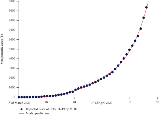
Data fitting to the reported cases in Saudi Arabia from March 02, 2020, till April 14, 2020, using model (6) and the nonlinear least-square method.

Figure 3.

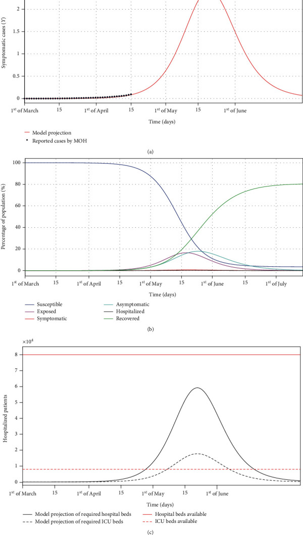
Numerical results of the SEYNHR model with the parameter listed in Table 1. (a) Shows the estimated number of symptomatic COVID-19 cases, with the published data by the Ministry of Health in Saudi Arabia of confirmed COVID-19 cases (blue circles). (b) Shows the estimated susceptible, exposed, symptomatic, asymptomatic, hospitalized, and recovered subpopulations. (c) Shows estimations of the hospitalized cases and the required ICU beds (black dashed line). The red line represents the number of hospital beds available, while the red dashed line represents the number of ICU beds available in Saudi Arabia.

5. Numerical Results and Discussion

To illustrate the numerical results, we take the initial population and subpopulations as Q(0) = 34218169, Y(0) = 2, S(0) = Q(0) − Y(0) = 34218167, and E(0) = N(0) = H(0) = R(0). The estimated values of parameters fitted from COVID-19 cases from March 02 till April 14 published by the Ministry of Health in Saudi Arabia (MOH) are presented in Table 1. Figure 3 shows the simulation of the model (6) with parameter values in Table 1. Figure 3(b) shows that about 18% of the entire Saudi population will be asymptomatic in the last week of May 2020, and about 17% will be exposed in the third week of May. The percentage of the entire population being symptomatic at any time will not exceed 1%, which is estimated to occur in the third week of May.

Moreover, as shown in Figure 3(c), about 60000 hospital beds and 18000 ICU beds are required (assuming 30% of the hospitalized cases need ICU [6]) immediately after the second week of May. As of April 2020, the Ministry of Health in Saudi Arabia designated 25 hospitals for COVID-19-infected patients with up to 80000 beds and 8000 intensive care unit (ICU) beds [15] and therefore extra 10000 ICU beds could be required.

The parameters β₁, β₂, and β₃ represent the impact of effective contact on the disease transmission as shown in Figures 4, 5, and 6. The effective contact rate from asymptomatic to susceptible β₂ has the greatest impact on the number of new COVID-19 symptomatic cases Y(t) as shown in Figure 5. This is because of the large number of asymptomatic cases in comparison to symptomatic cases in the same timescale as shown in Figure 3(b). Thus, social distancing (reduction of β₂) is an effective strategy to control the spread of the disease. The effective contact rate from hospitalized to susceptible β₃ has no impact on the number of new COVID-19 symptomatic cases Y(t) as shown in Figure 6 because of the small number of hospitalized cases in comparison to asymptomatic and symptomatic cases. Figure 7 shows that increasing the rate of asymptomatic becomes symptomatic K decreases the number of new COVID-19 symptomatic cases Y(t) because decreasing K implies increasing the contact time between individuals with COVID-19 (with no treatment) and susceptible individuals.

Figure 4.

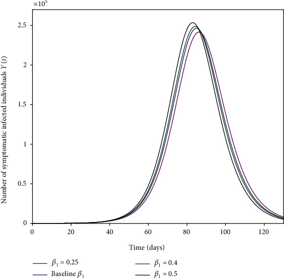
Effective contact rate from symptomatic to susceptible β₁ (a measure of social-distancing effectiveness) on the number of new COVID-19-infected cases Y(t). The baseline value of β₁ is as given in Table 1.

Figure 5.

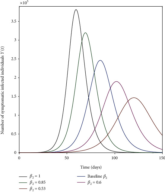
Effective contact rate from asymptomatic to susceptible β₂ (a measure of social-distancing effectiveness) on the number of new COVID-19-infected cases Y(t). The baseline value of β₂ is as given in Table 1.

Figure 6.

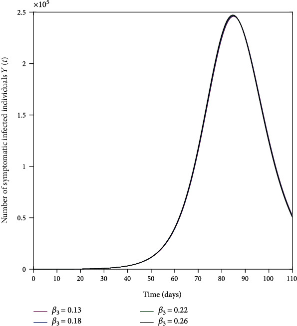
Effective contact rate from hospitalized to susceptible β₃ on the number of new COVID-19-infected cases Y(t). The baseline value of β₃ is as given in Table 1.

Figure 7.

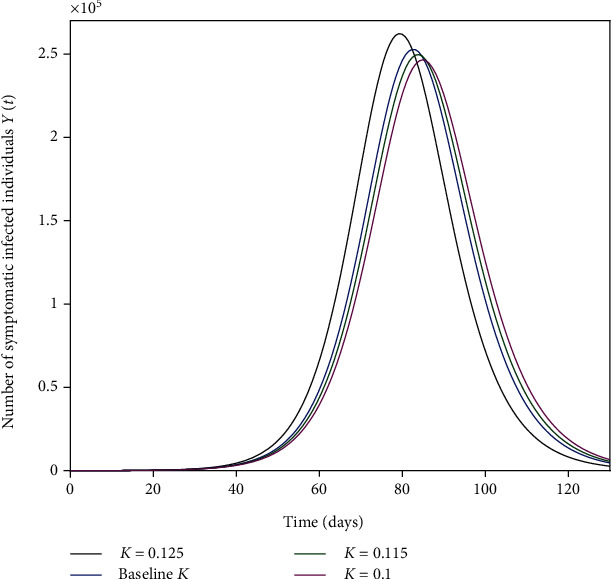
Impact of the rate of asymptomatic becomes symptomatic K on the number of new COVID-19-infected cases Y(t).

Based on estimated and measured parameter values, the basic reproduction number is estimated as R₀ ≈ 2.7. The variation of the basic reproduction number R₀ for different values of β₁ and β₂ and β₁ and K are shown in the heat maps in Figure 8. The upper heat map shows that decreasing the effective contact rate from symptomatic to susceptible β₁ and the effective contact rate from asymptomatic to susceptible β₁ will decrease the spread of the disease as R₀ decreases and vice versa. The lower heat map of Figure 8 shows that increasing K increases R₀ and vice versa. In reality, R₀ is not a biological constant; it could fluctuate daily depending on environmental and social factors such as the percentage of the entire susceptible population wearing a suitable medical mask and practicing physical distancing. In the literature, estimates of R₀ vary greatly: from 1 to 6 [13, 16–22] up to 26.5 [12]. This variation is because of the different assumptions and factors they had considered in their calculations.

Figure 8.

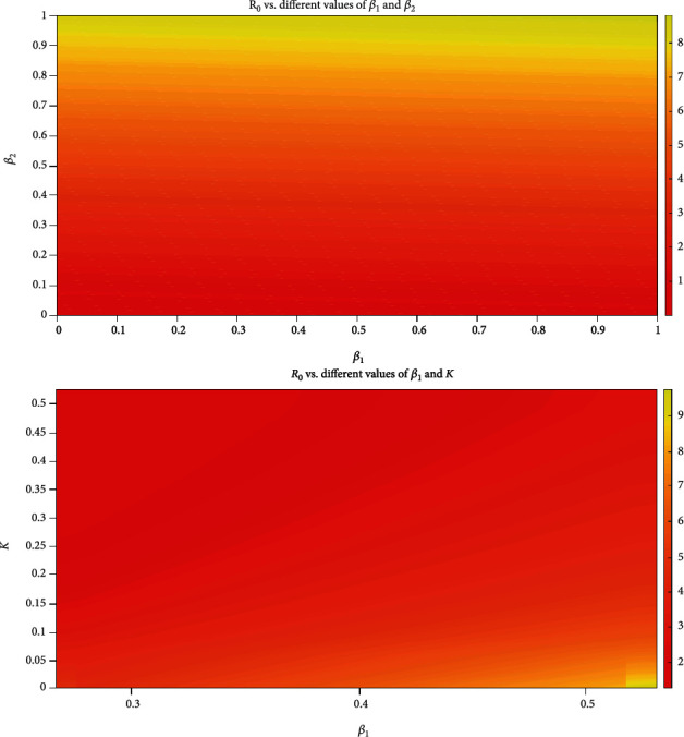
Heat maps showing the variation of R₀ for different parameter values: the upper heat map shows the variation of R₀ for different values for β₁ and β₂, and the lower heat map shows the variation of R₀ for different values for β₁ and K.

Parameters with the highest degree of uncertainty are the effective contact rates from symptomatic to susceptible β₁, from asymptomatic to susceptible β₂, and from hospitalized to susceptible β₃ (expected to be a fraction of β₁ because of the protective measures in hospitals); the rate of asymptomatic becomes symptomatic K as well as the mean asymptomatic infectious period Φ_N⁻¹.

The maximum estimated value of β₁ is 0.5 per day which is one half of the value reported by Li et al. [16]. This could be a reasonable estimation as we have not seen a similar scenario in Saudi Arabia after 5 weeks since reaching 100 confirmed cases on the 14th of March (week 7 since the first case) as we have seen in many other countries like China, America, and different European countries in the same timescale. This could be a result of the precautionary measures taken by the Saudi authorities, including the closure of schools and universities that started as early as March 08 (six days after the first confirmed COVID-19 case in Saudi Arabia).

6. Conclusion

The COVID-19 pandemic has rapidly spread out to most countries around the world. As of April 22, 2020, more than 12772 cases had been confirmed in Saudi Arabia alone. In this study, a mathematical model is formulated in order to study the transmission of COVID-19 in Saudi Arabia. Some basic properties of the model are presented in Section 3 including model positivity, boundedness, and local and global stability around the disease-free equilibrium. It is proven that the disease-free equilibrium is locally and globally stable when R₀ < 1. The model parameterized from COVID-19 confirmed cases reported by the Ministry of Health in Saudi Arabia (MOH) from March 02 till April 14, while some parameters are estimated from the literature. The numerical simulation showed that the model predicted infected curve is in good agreement to the real data of infected cases. An analytical expression of the basic reproduction number R₀ is obtained in Section 3, and the numerical value is estimated as R₀ ≈ 2.7.

The contribution of undocumented COVID-19 infections (asymptomatic cases) on the transmission of the disease deserves further studies and investigations. The obtained analytical expression of R₀, along with the numerical result in Figure 5, shows that asymptomatic transmission of COVID-19 could drive the growth of the pandemic in Saudi Arabia. Therefore, more testing and social distancing are needed to identify COVID-19 patients and to contain the spread of the disease.

Data Availability

The data used in my paper is the total number of confirmed cases of COVID-19 reported by the Ministry of Health in Saudi Arabia from the 2nd of March until the 21st of April 2020. Data supporting this paper are open and can be accessed through (in Arabic) Ministry of Health COVID 19 Dashboard. Saudi Arabia; 2020 (https://covid19.moh.gov.sa). Alternatively, data supporting this paper are open and can be accessed through (in English) Our World in Data; Oxford; 2020 (https://covid.ourworldindata.org/data/owid-covid-data.csv).

Conflicts of Interest

The author declares that he has no competing interests.

References

- 1.Ministry of health in Saudi Arabia. Covid-19 dashboard. 2020, https://covid19.moh.gov.sa.
- 2.Fraser C., Riley S., Anderson R. M., Ferguson N. M. Factors that make an infectious disease outbreak controllable. Proceedings of the National Academy of Sciences. 2004;101(16):6146–6151. doi: 10.1073/pnas.0307506101. [DOI] [PMC free article] [PubMed] [Google Scholar]
- 3.Peak C. M., Childs L. M., Grad Y. H., Buckee C. O. Comparing nonpharmaceutical interventions for containing emerging epidemics. Proceedings of the National Academy of Sciences. 2017;114(15):4023–4028. doi: 10.1073/pnas.1616438114. [DOI] [PMC free article] [PubMed] [Google Scholar]
- 4.Kang M., Song T., Zhong H., et al. Contact tracing for imported case of Middle East respiratory syndrome, China, 2015. Emerging infectious diseases. 2016;22(9):1644–1646. doi: 10.3201/eid2209.152116. [DOI] [PMC free article] [PubMed] [Google Scholar]
- 5.Hellewell J., Abbott S., Gimma A., et al. Feasibility of controlling COVID-19 outbreaks by isolation of cases and contacts. The Lancet Global Health. 2020;8(4):e488–e496. doi: 10.1016/S2214-109X(20)30074-7. [DOI] [PMC free article] [PubMed] [Google Scholar]
- 6.World Health Organization. Coronavirus disease (COVID-2019) situation reports. 2020. https://www.who.int/emergencies/diseases/novel-coronavirus-2019/situation-reports/
- 7.Li Q., Guan X., Wu P., et al. Early transmission dynamics in Wuhan, China, of novel coronavirus-infected pneumonia. New England Journal of Medicine. 2020;382(13):1199–1207. doi: 10.1056/NEJMoa2001316. [DOI] [PMC free article] [PubMed] [Google Scholar]
- 8.Van den Driessche P., Watmough J. Reproduction numbers and sub-threshold endemic equilibria for compartmental models of disease transmission. Mathematical biosciences. 2002;180(1-2):29–48. doi: 10.1016/S0025-5564(02)00108-6. [DOI] [PubMed] [Google Scholar]
- 9.Ullah S., Atlaf Khan M. Modeling the impact of non-pharmaceutical interventions on the dynamics of novel coronavirus with optimal control analysis with a case study. Solitons and Fractals. 2020;139:p. 110075. doi: 10.1016/j.chaos.2020.110075. [DOI] [PMC free article] [PubMed] [Google Scholar]
- 10.LaSalle J. P. The stability of dynamical systems. Philadelphia, PA, USA: Society for Industrial and Applied Mathematics; 1976. [DOI] [Google Scholar]
- 11.General authority for statistics in Saudi Arabia. Statistics library. 2020, https://www.stats.gov.sa/en/43.
- 12.Aguilar J. B., Faust J. S., Westafer L. M., Gutierrez J. B. Investigating the impact of asymptomatic carriers on COVID-19 transmission. COVID-19 Publications by UMMS Authors. 2020, https://escholarship.umassmed.edu/covid19/6. [DOI] [Google Scholar]
- 13.Atlaf Khan M., Antangana A. Modeling the dynamics of novel coronavirus (2019-nCov) with fractional derivative. Alexandria Engineering Journal. 2020;59 [Google Scholar]
- 14.Ullah S., Atlaf Khan M., Farooq M., Gul T. Modeling and analysis of tuberculosis (TB) in Khyber Pakhtunkhwa, Pakistan. Mathematics and Computers in Simulation. 2019;165:181–199. doi: 10.1016/j.matcom.2019.03.012. [DOI] [Google Scholar]
- 15.World Health Organization. Regional Office for the Eastern Mediterranean. 2020.
- 16.Li R., Pei S., Chen B., et al. Substantial undocumented infection facilitates the rapid dissemination of novel coronavirus (SARS-CoV-2) Science. 2020;368(6490):489–493. doi: 10.1126/science.abb3221. [DOI] [PMC free article] [PubMed] [Google Scholar]
- 17.Wu P., Hao X., Lau E. H. Y., et al. Real-time tentative assessment of the epidemiological characteristics of novel coronavirus infections in Wuhan, China, as at 22 January 2020. Eurosurveillance. 2020;25(3) doi: 10.2807/1560-7917.ES.2020.25.3.2000044. [DOI] [PMC free article] [PubMed] [Google Scholar]
- 18.Yanga J., Zhenga Y., Goua X. Prevalence of comorbidities and its effects in coronavirus disease 2019 patients: a systematic review and meta-analysis. International Journal of Infectious Diseases. 2020;94:91–95. doi: 10.1016/j.ijid.2020.03.017. [DOI] [PMC free article] [PubMed] [Google Scholar]
- 19.Guan W. J., Ni Z. Y., Hu Y., et al. Clinical characteristics of 2019 novel coronavirus infection in China. medRxiv; 2020. [DOI] [Google Scholar]
- 20.Wu J. T., Leung K., Leung G. M. Nowcasting and forecasting the potential domestic and international spread of the 2019-nCoV outbreak originating in Wuhan, China: a modelling study. The Lancet. 2020;395(10225):689–697. doi: 10.1016/S0140-6736(20)30260-9. [DOI] [PMC free article] [PubMed] [Google Scholar]
- 21.Shen M., Peng Z., Xiao Y., Zhang L. Modelling the epidemic trend of the 2019 novel coronavirus outbreak in China. bioRxiv; 2020. [DOI] [PMC free article] [PubMed] [Google Scholar]
- 22.Read J. M., Bridgen J. R. E., Cummings D. A. T., Jewell C. P. Novel coronavirus 2019-nCoV: early estimation of epidemiological parameters and epidemic predictions. medRxiv; 2020. [DOI] [PMC free article] [PubMed] [Google Scholar]
- 23.Lauer S. A., Grantz K. H., Bi Q., et al. The incubation period of coronavirus disease 2019 (COVID-19) from publicly reported confirmed cases: estimation and application. Annals of Internal Medicine. 2020;172(9):577–582. doi: 10.7326/M20-0504. [DOI] [PMC free article] [PubMed] [Google Scholar]
- 24.Nishiura H., Kobayashi T., Yang Y., et al. The rate of underascertainment of novel coronavirus (2019-ncov) infection: estimation using japanese passengers data on evacuation flights. 2020. [DOI] [PMC free article] [PubMed]
- 25.Zhou F., Yu T., Du R., et al. Clinical course and risk factors for mortality of adult inpatients with COVID-19 in Wuhan, China: a retrospective cohort study. The Lancet. 2020;395(10229):1054–1062. doi: 10.1016/S0140-6736(20)30566-3. [DOI] [PMC free article] [PubMed] [Google Scholar]
- 26.Baud D., Qi X., Nielsen-Saines K., Musso D., Pomar L., Favre G. Real estimates of mortality following COVID-19 infection. The Lancet Infectious Diseases. 2020;20(7):p. 773. doi: 10.1016/S1473-3099(20)30195-X. [DOI] [PMC free article] [PubMed] [Google Scholar]
Associated Data
This section collects any data citations, data availability statements, or supplementary materials included in this article.
Data Availability Statement