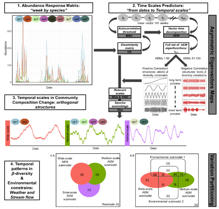
Figure 1.

Workflow to analyze Culicoides temporal dynamic and its drivers: the sequence of steps from collecting Culicoides field abundance data, drawing temporal scales and identifying β-diversity scales and their relatedness with environmental variability. White filled boxes outline the aim for each analysis, and dark gray boxes mention the statistical tools used. Step 1 shows the temporal dynamic of the observed abundance in a nine-species virtual community; therefore, it was the response matrix informing weekly community composition. Step 2: the sampling temporal profile was thrown to spectral decomposition by asymmetric eigenvectors maps (AEMs) after accounting for the dependency between weeks (autocorrelation threshold). The resulting AEMs were half splitting in positive and negative correlation structures, and a subset was selected by their suitability to model temporal patterns in the observed abundance matrix. Selected subsets were arranged in groups representing broad to narrow temporal waves, hereafter referred to as temporal submodels. Step 3: the community composition change was modeled with each temporal submodel to assess the fitting of the temporal scale on the observed species abundance matrix. The assemblage of species contributing on each significant temporal scale was untangled by the correlation between each species abundance and Lc for each RDA_axis. Step 4: the contribution of the temporal submodels and environmental variables to explain the amount of variation was visualized by Venn diagrams after hierarchical variation partitioning analysis. Since temporal scales were nested, even when there were orthogonal structures, both diagrams show intersection areas between temporal submodels as a hierarchical overlapping pattern. Letters inside diagrams are R²_adj for each unique and intersection fraction in the variation partitioning table (as were introduced in Section 2.4: Culicoides β-diversity temporal profile; equations for the fractions are detailed in [84]). AEM: asymmetric eigenvectors maps; AEMs: AEM eigenfunctions; FWD: forward selection; Hd: Hellinger’s distance; Lc: linear combinator scores from an RDA_axis; MMC: multivariate Mantel correlogram; RDA: redundancy analysis; Rho: Rank Spearman correlation; R²_adj: adjusted determination coefficient. This scheme was adapted considering [9,83] (Figure 1).