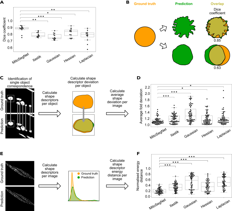
Figure 3.
MitoSegNet's Pixelwise Accuracy Outperforms Non-Deep Learning Segmentation Methods
(A) The average dice coefficient achieved with the MitoSegNet is significantly higher than with the four other segmentation approaches. The data was statistically evaluated by using the Kruskal-Wallis test followed by a Dunn's multiple comparisons test.
(B) The dice coefficient is limited as a predictor of morphological segmentation performance: A dice coefficient close to 1.0 does not guarantee correct prediction of morphology. Contrary, a low dice coefficient does not rule out an accurate shape prediction. Ground truth segmentation is shown in orange, and the predicted segmentation in green.
(C) To gain insight into how accurately the shape of ground truth objects is predicted, five object shape descriptors (area, eccentricity, aspect ratio, perimeter, and solidity) are compared by calculating the fold deviation. Predicted objects that correspond to more than one ground truth object (or vice versa) are excluded from this analysis.
(D) The MitoSegNet shows the lowest average fold deviation between predicted and ground truth object shape descriptors. The data were statistically evaluated by first testing for normality using D'Agostino's K-squared test and then subsequently using the Kruskal-Wallis test followed by a Dunn's multiple comparisons test. N = 60.
(E) To determine the total morphological prediction accuracy, the same five shape descriptors were measured for each image. The descriptor distributions in the ground truth and predicted images were statistically evaluated for differences by calculating the energy distances between predicted and ground truth distribution. The energy distances for each shape descriptor and image were normalized prior to statistical analysis.
(F) The MitoSegNet shows the lowest normalized energy distance, statistically outperforming all other segmentation approaches. The data were first tested for normality using the D'Agostino's K-squared. After determining that all distributions were non-parametric, a Kruskal-Wallis test was used followed by a Dunn's multiple comparisons test. N = 60. ∗p < 0.05, ∗∗0.001 < p < 0.01, ∗∗∗p < 0.001 for (A), (D) and (F).

