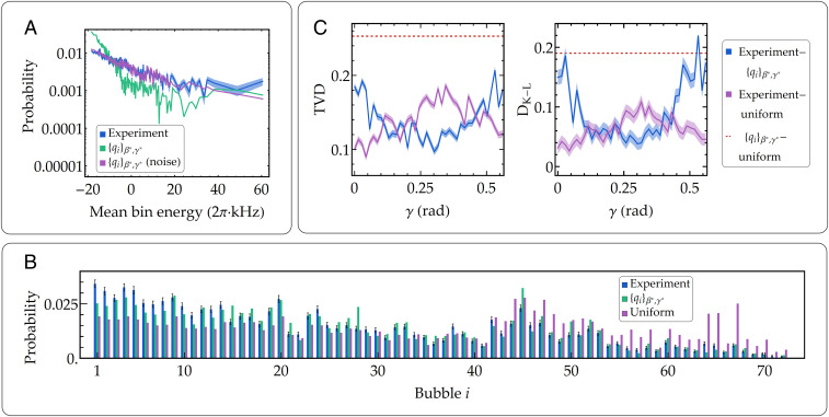
Fig. 4.

Sampling from $p=1$ QAOA. (A) Eigenstate probability histogram for 12 qubits with $B=0$. The numerical histogram is computed by decomposing the ideal QAOA output state on the $\left\{\left|x_i\right.⟩\right\}$ basis. We performed 10,800 measurements to oversample the Hilbert space of dimension 2^N = 4,096 at the optimal parameters ${\beta }^{*}=0.25$ and ${\gamma }^{*}=0.31$. The 4,096 eigenstates are grouped in bins of 20 for clarity purposes. The uncertainty bands follow the multinomial distribution SD. Here, $J_0/2\pi =0.33$ kHz (see SI Appendix, Noise Sources for details). (B) Histogram of coarse-grained distributions (see Combinatorial Optimization for details) comparing data, theory, and the uniform distribution. The error bars here also represent the SD of the multinomial distribution. (C) TVD and Kullback–Leibler divergence as a function of $\gamma$, keeping $\beta$ fixed at the optimal value (1,350 shots per time step). The nonzero TVD value of the violet curve at $\gamma =0$ is due to state preparation and detection errors, as well as undersampling (SI Appendix). The distance from the uniform distribution increases as the $\gamma$ parameter reaches the optimal point ${\gamma }^{*}$. Dashed lines are the comparison between the ideal QAOA distribution ${\left\{q_i\right\}}_{{\beta }^{*},{\gamma }^{*}}$ and the uniform distribution. The uncertainty bands are based on the aforementioned error in the probability of each state bubble for the experimental distribution, propagated to the TVD and the ${\mathrm{D}}_{\mathrm{K}-\mathrm{L}}$, according to Eq. 4 (data taken on system 2)..