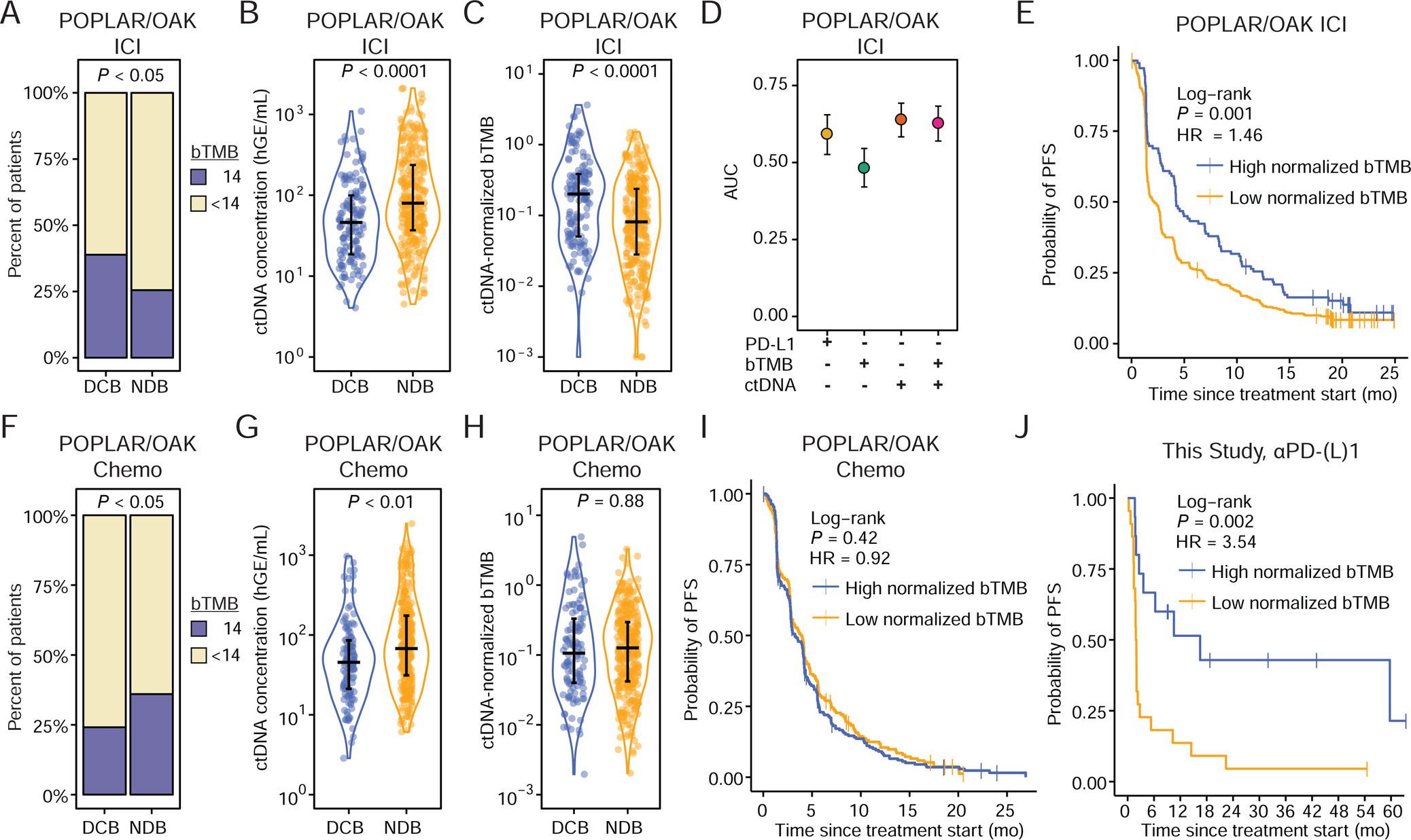
Figure 2: Pre-treatment ctDNA-normalized tumor mutation burden predicts response to ICI.

A) Outcomes of PD-L1 blockade treated patients from the POPLAR/OAK Cohort (Gandara et al., 2018) (POPLAR/OAK ICI Cohort) stratified by high bTMB/MB (≥14) and low bTMB/MB (<14). P-value calculated by two-sided Fisher’s Exact Test (DCB n = 139; NDB n = 290).
B) Pre-treatment ctDNA concentration (haploid genome equivalents per mL of plasma, hGE/mL) and C) ctDNA-normalized bTMB (norm. bTMB) in POPLAR/OAK ICI Cohort. P-values were calculating using a Wilcoxon test.
D) Area under the curve (AUC) for individual parameters in immunotherapy patients generated by leave-one-out cross-validation (LOOCV) ROC analysis.
E) Probability of PFS for high norm. bTMB (median = 4.14 mo.) and low norm. bTMB (median = 2.16 mo.) PD-L1 blockade patients stratified by the LOOCV-identified optimal cut-point in the POPLAR OAK ICI Cohort (n = 429).
F) Outcomes of chemotherapy treated patients from the POPLAR/OAK Cohort (Gandara et al., 2018) (POPLAR/OAK Chemo Cohort) stratified by high bTMB/MB (≥14) and low bTMB/MB (<14). P-value calculated by two-sided Fisher’s Exact Test (DCB n=118; NDB n = 306).
G) Pre-treatment ctDNA concentration and H) norm. bTMB (POPLAR/OAK Chemo Cohort) in chemotherapy patients. P-values were calculated using a Wilcoxon test.
I) Probability of PFS for high norm. bTMB (median = 3.25 mo.) and low norm. bTMB (median = 4.00 mo.) chemotherapy patients stratified by the LOOCV-identified optimal cut-point in the POPLAR/OAK Chemo Cohort (n = 424).
J) Probability of PFS for high norm. bTMB (median = 16.49 mo.) and low norm. bTMB (median = 1.92 mo.) patients who received single-agent PD-(L)1 blockade in this study, exclusive of the DIREct Validation Cohort (n = 37) stratified by the cut-point of norm. bTMB identified in the POPLAR/OAK ICI Cohort. See also Figure S2.
