
Figure 3. Impact of saccade amplitude.
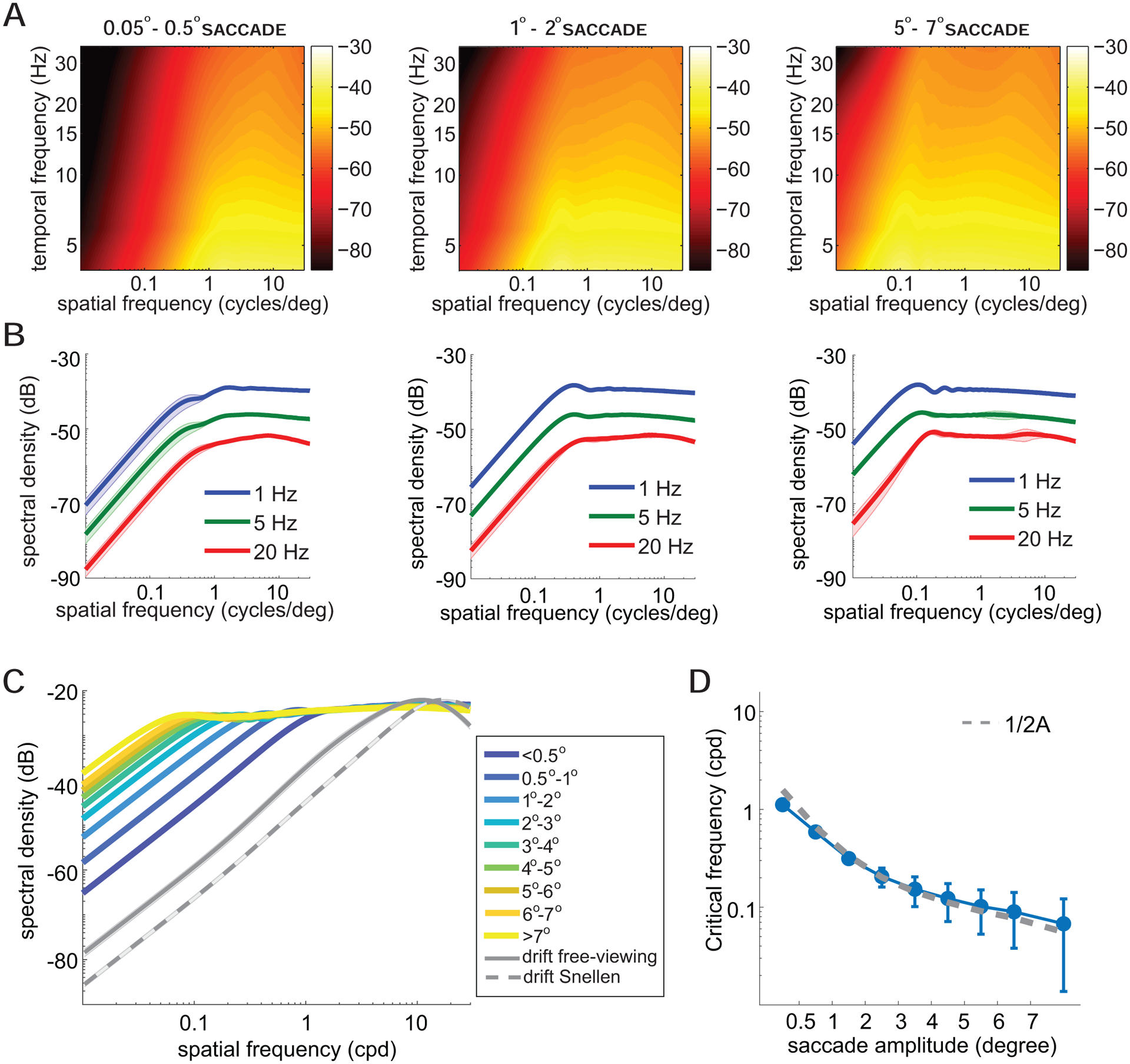
(A-B) The analysis of Figure 2 is here conducted for saccades in three different amplitude ranges. Graphical conventions are as in Figure 2. The full spatiotemporal spectra are in A, and sections at selected temporal frequencies in B.
(C) Changes in power with saccade amplitude. Each curve represents the total power within the temporal range of human sensitivity [38] by saccades of a given amplitude. Shaded areas represent SEM across subjects. For comparison, the panel also shows the power of the modulations resulting from the inter-saccadic eye drifts recorded both in the experiments of this study and during examination of a 20/20 line in a Snellen chart (data from Intoy and Rucci [40]). (D) Critical spatial frequency, the frequency separating whitening and saturation regimes, as a function of saccade amplitude. This value was estimated from the curves in C, following the procedure described in Figure 2C. Experimental data are well approximated by the function 1/2A, where A is the saccade amplitude. Error bars represent one standard deviation across temporal frequencies.