

Abstract
The biological complexity reflected in histology images requires advanced approaches for unbiased prognostication. Machine learning and particularly deep learning methods are increasingly applied in the field of digital pathology. In this study, we propose new ways to predict risk for cancer‐specific death from digital images of immunohistochemically (IHC) stained tissue microarrays (TMAs). Specifically, we evaluated a cohort of 248 gastric cancer patients using convolutional neural networks (CNNs) in an end‐to‐end weakly supervised scheme independent of subjective pathologist input. To account for the time‐to‐event characteristic of the outcome data, we developed new survival models to guide the network training. In addition to the standard H&E staining, we investigated the prognostic value of a panel of immune cell markers (CD8, CD20, CD68) and a proliferation marker (Ki67). Our CNN‐derived risk scores provided additional prognostic value when compared to the gold standard prognostic tool TNM stage. The CNN‐derived risk scores were also shown to be superior when systematically compared to cell density measurements or a CNN score derived from binary 5‐year survival classification, which ignores time‐to‐event. To better understand the underlying biological mechanisms, we qualitatively investigated risk heat maps for each marker which visualised the network output. We identified patterns of biological interest that were related to low risk of cancer‐specific death such as the presence of B‐cell predominated clusters and Ki67 positive sub‐regions and showed that the corresponding risk scores had prognostic value in multivariate Cox regression analyses (Ki67&CD20 risks: hazard ratio (HR) = 1.47, 95% confidence interval (CI) = 1.15–1.89, p = 0.002; CD20&CD68 risks: HR = 1.33, 95% CI = 1.07–1.67, p = 0.009). Our study demonstrates the potential additional value that deep learning in combination with a panel of IHC markers can bring to the field of precision oncology.
Keywords: gastric cancer, deep learning, survival analysis, computational pathology, tumour infiltrating immune cells, Ki67
Introduction
A tumour and its microenvironment consist of various cell types which interact in complex ways [1]. In addition to cancer cells, immune cells of both lymphoid (e.g. cytotoxic T cells) and myeloid lineage (e.g. macrophages) can be found in the tumour stroma. The distinct composition of cells and their interaction with each other are thought to play an important role in tumour development, tumour growth, metastasis and patient prognosis in various cancer types [2, 3].
Traditionally, pathologists estimate quantities of cell types, such as Ki67 positive cells for the grading of neuroendocrine tumours, by counting positive cells in a predefined number of selected fields of view [4]. In some tumour types, classification systems such as grading, scoring and tumour subtyping allow for prognostication. However, such approaches suffer from subjectivity, intra‐ and inter‐observer variability and are biased by prior knowledge [5].
With the recent boost in deep learning methodology, time‐consuming and tedious tasks such as cell and region detection/classification are increasingly being automated [6, 7, 8]. Deep learning models such as convolutional neural networks (CNNs) learn a hierarchical set of filters (convolutions), guided by a so‐called ‘loss function’ that measures the difference between ground truth and predictions.
Instead of using knowledge‐based features (based on the detected regions and cells) for patient stratification, end‐to‐end learning aims at directly associating images with survival data. Accordingly, the loss function needs to take into account the characteristics of survival data, i.e. the non‐Gaussian distribution and censoring events. Straightforward dichotomisation based on the median survival or regression on survival time ignores either time or event. In contrast, Cox regression models the influence of covariates on survival via the proportional hazards condition [9]. In classical Cox regression models, features are linearly combined and complex non‐linear relationships are neglected. Faraggi and Simon were the first to replace the linear form by a non‐linear neural network as input in the loss function based on the Cox model (Cox loss) and applied their network to a prostate cancer dataset [10]. Yousefi et al demonstrated that deep survival models in combination with Bayesian optimisation can be successfully applied in a large‐scale genomic profile project [11]. In a study by Mobadersany et al, patient outcomes were predicted from H&E‐stained whole slide images of gliomas using a CNN that was driven by a Cox loss [12]. In another study, Bychkov et al trained recurrent architectures to directly predict colorectal cancer outcome based on haematoxylin and eosin (H&E)‐stained tissue microarray (TMA) images using cross‐entropy loss (5‐year survival) [13]. As an alternative to minimising the Cox loss, Mayr et al proposed optimising the concordance index for time‐to‐event data to identify molecular signatures with gradient boosting [14, 15].
In the study presented here, we used CNNs to automatically learn time‐to‐event outcomes from TMA images from a Japanese patient cohort with gastric cancer. Advancing previous work, which focused on H&E sections, we analysed immunohistochemical (IHC) stains for CD8 (cytotoxic T cells), CD20 (pan‐B cells), CD68 (pan‐macrophages) and Ki67 (proliferating cells) by training CNNs with three different survival‐specific loss functions: (1) the Cox loss, (2) a new CNN‐adapted concordance loss and (3) a new loss that maximises the logrank test statistic.
Our CNN‐derived risk scores made a significant contribution in multivariable Cox regression and outperformed cell density features as well as scores derived from models using binary (median cancer‐specific survival time) classification. Computing risk heat maps allowed us to identify tissue regions associated with low or high risk for cancer‐specific death.
Materials and methods
Patient cohort
In total, the dataset consisted of digital images of IHC stained TMAs from 248 patients from a gastric cancer patient cohort with locally advanced disease who had surgery at the Kanagawa Cancer Center Hospital, Yokohama, Japan [16].
Two tissue cores (1.2 mm diameter each) from an area of highest tumour cell density were used for TMA construction and served as our regions of interest. The 4 μm TMA sections were stained for the immune cell markers CD68 (pan‐macrophages), CD8 (cytotoxic T cells) and CD20 (pan B cells); the proliferation marker Ki67; and H&E, as described previously [16]. Sections were scanned at ×40 magnification using an Aperio XT (Aperio Technologies, Vista, CA) digital slide scanner. All artefacts such as air bubbles, blurry regions and folds were manually annotated and excluded from analyses. After quality control, 90% of patients had two cores available for each stain, the remaining 10% a single one. We used cancer‐specific survival time from surgery for analyses (median follow up time 86 months, range from 3.3 to 150 months). As patients in this cohort were either treated by surgery only or surgery followed by adjuvant chemotherapy, we confirmed that there was no interaction between our risk scores and treatment using Cox regression analysis. Clinicopathological characteristics of the cohort can be found in supplementary material, Table S1. Studies were approved by Local Research Ethics Committees.
Technical workflow: from TMA images to risks
In this study, we aimed to identify survival related features from images. The data and high‐level workflow overview are shown in Figure 1. Image patches (160 × 160 pixels at ×20 magnification corresponding to 80 × 80 μm) were extracted from the TMA cores in the training set for each stain and fed into the CNN training. During training, risk‐relevant features were automatically extracted in the CNN layers. The last, fully connected layer then returned for each patch a single risk value that was related to patient cancer‐specific survival. The learning process was guided by a specific loss function, which considered the time‐to‐event and censoring status. In addition to the Cox loss, we developed two new CNN loss functions: the ‘Uno loss’ which maximised the concordance index and the ‘Logrank loss’ which optimised the logrank test statistic. Trainings were performed for each stain separately.
Figure 1.
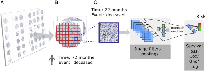
(A) TMA images acquired from a Japanese gastric cancer cohort. (B) All cores of a given patient are tiled into patches. Both survival time and event are forwarded from the patient to the patch level. (C) A convolutional neural network is trained to predict survival risks from a given input patch. Parameter estimation is guided by one of three survival loss functions: Cox, Uno or Logrank loss.
During prediction, unseen TMA cores from the test set were tiled into patches and forwarded in the CNN. To aggregate data to patient level, we restricted ourselves to computing only the median risk score of all patches per patient and stain, which avoids multiple testing issues (median as a descriptive statistic of the risk distribution, see supplementary material, Figure S1). Two stains were combined by adding their respective single stain risk values. Due to the medium size of the patient cohort (n = 248) and the lack of an independent validation set, we used a pre‐validation procedure to assess the performance of different IHC‐associated risk factors (see supplementary material, Figure S2).
Deep learning: network training and prediction
As network architecture, we used a slightly modified GoogLeNet [17] to tradeoff network size against reported classification accuracy considering our cohort size and computational costs (see supplementary material, Appendix S1.1). For the same reason, we did not tune the network architecture or patch size and resorted to default values. In the default version, the next to the last layer defines a 1024‐dimensional feature vector x. We changed the final fully connected layer from a 1000 class output to a single output. x is then multiplied by a weight vector β ɛ ℝ1024 to give the scalar risk value xTβ.
Loss functions
All three of the following loss functions take into account that survival data are a composite of a survival time T and an event status (deceased or censored).
Cox loss: In case of the Cox model, the loss is given by the negative log partial‐likelihood of the survival data given the image patches (see supplementary material, Appendix S1.2 for more details).
Uno loss: This loss is based on the concordance index C ‐ index = P(ri > ri|Ti < Tj), where r i, r j are the risks for case i, j and T i, T j are the corresponding cancer‐specific survival times. The C‐index is 1 in the case of perfect ordering and 0.5 for random sorting. Uno et al proposed a consistent and asymptotically normal estimator of the C‐index which we employed for our loss function [14]. In contrast to Mayr et al [15], we did not use gradient boosting with linear base learners but used non‐linear CNN to retrieve the feature vectors xi, xj from the input image patches (see supplementary material, Appendix S1.3 for more details).
Logrank loss: The logrank test is a non‐parametric test to compare right‐skewed and censored survival data. As loss function, we resorted to its test statistic, which we transformed into a smooth function. The input feature vectors which enter the loss function were again retrieved by forward passing the image patches (see supplementary material, Appendix S1.4 for more details).
Cell densities
To compare the prognostic value of our CNN‐derived scores with a conventional cell segmentation approach, we segmented individual cells and classified them into marker positive or marker negative. Segmentation was done by identifying foreground regions via maximally stable extremal regions (MSER) [18] followed by the application of geometric descriptors such as convex hull‐based filterings. Subsequently, the detected objects were classified into marker positive or negative by their mean blue to red ratio. Next, a slide‐specific visual context random forest was trained on these classified candidates to return posterior maps to perform the final detection steps [19]. Positive cell densities were calculated as the number of positive cells per patient divided by the core area per patient. For combined features, two such densities were either multiplied or added.
Statistical analyses
We included age, gender, body mass index (BMI), histological phenotype according to Lauren classification, TNM or pT, which is more locally confined than TNM, as co‐variables into the multivariable Cox regression. The significance level for statistical tests was chosen as 0.05. To assess the prognostic value of our risk scores (median value of all patches per patient), we stratified patients into low‐risk and high‐risk using the median cohort risk score as a threshold. Kaplan–Meier curves were generated and the difference in survival between the low‐risk and high‐risk group was assessed by the logrank test. Risks from two different stains were combined by adding them (see supplementary material, Appendix S1.5).
Statistical analyses such as univariable and multivariable Cox regressions and logrank tests were performed using the R package survival (v2.41.3). CNN training and prediction were run in TensorFlow/keras (v.1.10.0) on a NVidia K80 graphics card (see supplementary material, Appendix S1.6 for more details).
Results
Risk heat map analysis
Similarly to Yousefi et al [11], we used risk heat maps to visualise structures in the images which the network has learned to associate with specific risks. During prediction, each TMA core was tiled into patches and each patch was forwarded through the network. The final layer returned the risk of the respective patch, which was then used for a colour‐coded transparent overlay onto the original image (ranging from green for low risk to red for high risk). These risk maps allowed a pathologist to visually evaluate the network output thereby enabling the identification of patterns of interest and to compare regions with different risks.
Overall, the risk maps for the Cox/Uno/Logrank losses were visually comparable, as shown for a representative core in Figure 2A. Across all markers, epithelial regions were easily distinguishable due to a consistently higher risk compared to other regions such as stroma and immune cell clusters.
Figure 2.
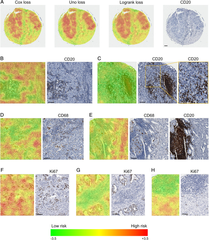
Risk maps for the markers CD20, CD68 and Ki67 with low and high risks indicated in green and red, respectively. (A) Comparison of risk maps for the different loss functions for a core stained for CD20. (B,C) Representative risk maps for CD20. (B) Tumour epithelium is associated with a higher risk than stroma with a low density of CD20(+) cells. Stroma densely populated with CD20(+) cells has an even lower risk. (C) B cell clusters as well as CD20(+) cells infiltrating the epithelium are regarded as low risk. (D,E) Representative risk maps for CD68. (D) A high risk is predicted for epithelial cells with a tendency towards lower risks in regions infiltrated by CD68(+) cells. Infiltrated stroma is associated with low risks independent of CD68(+) cell densities. (E) Immune cell clusters that may contain CD68(+) cells are associated with low risks. Visual inspection of the corresponding core stained for CD20 reveals B cell clusters. (F,G,H) Representative risk maps for Ki67. (F) Epithelium is associated with high risks, with a decreased risk for regions dominated by Ki67(−) cells compared to Ki67(+) cells. (G) Immune cells in the stroma are linked to low risks. (H) Immune cell clusters (mostly Ki67(−) cells) are detected as low‐risk regions. They are often B cell clusters as revealed by comparison with the corresponding region stained for CD20 (not shown). If not stated otherwise, risks for the Uno loss are shown. Scale bars indicate 100 μm.
Qualitative analysis of the risk maps for CD20 images identified regions of tumour stroma with high densities of CD20(+) cells to be associated with lower risks than stromal regions with low densities of CD20(+) cells (see Figure 2B). B cell clusters were consistently assigned low risks, as shown in Figure 2C. Epithelial regions devoid of CD20(+) cells were identified as high risk (see Figure 2B), while infiltrating B cells lowered the risk (see Figure 2C).
In CD68 images, epithelial regions were associated with high risks tending towards lower risks in the presence of infiltrating CD68(+) cells, as depicted in Figure 2D. In contrast, tumour stroma densely populated with CD68(+) or CD68(−) immune cells was identified as low risk. The same applied for immune cell clusters. They often contained only few CD68(+) cells, and comparison with the corresponding CD20‐stained core revealed that the clusters were frequently dominated by B cells (see Figure 2E).
The interpretation of Ki67 associated risk maps was challenging due to the fact that both epithelial and immune cells can be Ki67 positive. Visual inspection suggested that immune cells were rarely Ki67 positive in this cohort. Epithelial regions with high percentages of Ki67(+) tumour cells were mostly associated with higher risks in comparison with regions dominated by Ki67(−) tumour cells (see Figure 2F). As seen in Figure 2G, lymphocytes in the tumour stroma, mainly Ki67(−), were detected as low‐risk structures compared to the tumour epithelium. Similarly to CD68, immune cell clusters were predicted as low risk in Ki67‐stained images (see Figure 2H). Only very few of these immune cells were Ki67(+), but they were often CD20(+) as confirmed visually.
Qualitatively, CD8 risks turned out to be inversely correlated with the density of epithelium‐infiltrating CD8(+) cells. Additionally, immune cell clusters, partly CD8(+), were confirmed to be low‐risk regions as for the other markers.
Stratification of the cohort with CNN‐based risk features
The results from univariable cancer‐specific survival analysis for all single stains (CD8, CD20, CD68 and Ki67) and pairs of stains for each loss function are summarised in Table 1. We observed that for CD8 and Ki67 none of the loss functions generated a significant patient stratification, whereas the Cox loss was able to stratify the cohort with all other univariable and bivariable scores. Figure 3 shows corresponding Kaplan–Meier curves for the three most significant P values using the Cox loss.
Table 1.
Logrank test P values for single and combined risk features for all three losses.
| Logrank test P values | |||
|---|---|---|---|
| Risk/loss | Cox | Uno | Logrank |
| Ki67 | ≥0.05 | ≥0.05 | ≥0.05 |
| CD8 | ≥0.05 | ≥0.05 | ≥0.05 |
| CD20 | 0.0159 | 0.00549 | 0.0108 |
| CD68 | 0.02 | 0.00707 | 0.0157 |
| Ki67&CD8 | 0.0268 | ≥0.05 | 0.0374 |
| Ki67&CD20 | <0.001 | 0.00536 | 0.00397 |
| Ki67&CD68 | 0.00697 | <0.001 | 0.00277 |
| CD8&CD20 | 0.0390 | 0.0376 | ≥0.05 |
| CD8&CD68 | 0.0196 | ≥0.05 | ≥0.05 |
| CD20&CD68 | 0.00847 | <0.001 | <0.001 |
The cohort was split into low‐risk and high‐risk arms based on the respective median cohort risk score per stain. Significant P values (<0.05) are shown in bold font.
Figure 3.
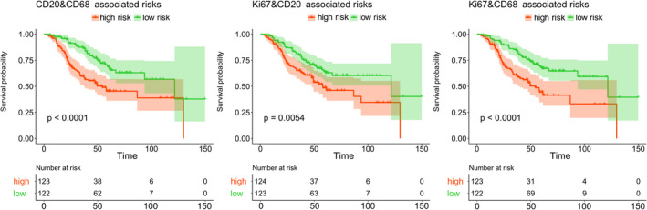
Kaplan–Meier plots (Uno loss) showing stratification of the cohort into low‐ and high‐risk arms. The groups were retrieved by thresholding the respective feature based on the cohort median.
All three loss variants returned consistent prognostic logrank test outcomes. P values for both Ki67‐ and CD8‐associated risk scores were non‐significant irrespective of the type of loss function (all p > 0.05). In contrast, CD20‐ and CD68‐associated risks had similar significant P values. Regarding combined risks, Ki67&CD8 was still only slightly below 0.05 for two of the three loss functions. Linking Ki67 with CD20 returned better P values than the single markers. CD8‐associated risks decreased the prognostic values of CD20 and CD68. Combining CD20 and CD68 instead, which already performed well as individual scores, even improved the stratification (Uno: CD20: p = 0.0055, CD68: p = 0.007 versus CD20&CD68: p = 9.22e−5). Hence, scores involving CD20‐ or CD68‐associated risks outperformed the ones involving CD8.
Correlation to clinical covariables
To further investigate the association between our IHC‐based risk scores and cancer‐specific survival while correcting for other clinical covariables, we performed multivariable Cox regressions. We included age, gender, BMI, histological phenotype according to Lauren classification (categorised as intestinal, diffuse or mixed) and TNM (see supplementary material, Table S2). Kaplan–Meier curves for the cohort stratified by TNM are shown in supplementary material, Figure S3. Whereas the survival CNN was restricted to information extracted from locally confined TMA cores from the primary tumour, the clinicopathological variable TNM additionally included information from regional lymph nodes (pN) and distant metastasis (pM). As shown in Table 2, combined risks including Ki67, CD20 and/or CD68 had hazard ratios (HRs) significantly larger than 1, including in the presence of the clinical covariables (Ki67&CD20: HR = 1.364, p = 0.013; CD20&CD68: HR = 1.338, p = 0.009; Ki67&CD68: HR = 1.473, p = 0.002; all for Logrank loss). Age, gender and BMI never appeared as relevant factors and thus are omitted in Table 2 (see supplementary material, Tables S3.1–3.4 for the complete tables). As expected, TNM stage was significant (stage III versus stage II: HR > 3.091, p < 0.8.2e−5). In each Cox regression result, Logrank loss‐based risk scores and Uno loss‐based risk scores outperformed Cox risk scores. Similar to the median‐based logrank test results, single‐marker risks for Ki67 and CD8 were either not or only slightly significant (see supplementary material, Table S3.2).
Table 2.
HRs for multivariable Cox regressions including the respective risk and TNM stage. Results for age, gender, BMI and Lauren classification are not shown as they were not significant (see supplementary material, Table S3.1).
| Multivariable Cox regression | |||||||||
|---|---|---|---|---|---|---|---|---|---|
| Cox | Uno | Logrank | |||||||
| HR | 95% CI | P value | HR | 95% CI | P value | HR | 95% CI | P value | |
| CD20&CD68 risk | 1.356 | 1.0, 1.84 | 0.049 | 1.27 | 1.02, 1.57 | 0.029 | 1.338 | 1.07, 1.67 | 0.009 |
| TNM stage III versus II | 3.342 | 1.9, 5.86 | <0.001 | 3.34 | 1.91, 5.84 | <0.001 | 3.231 | 1.84, 5.66 | <0.001 |
| TNM stage IV versus II | 6.851 | 2.98, 15.78 | <0.001 | 6.628 | 2.86, 15.34 | <0.001 | 6.56 | 2.87, 15.0 | <0.001 |
| Ki67&CD20 risk | 1.282 | 0.94, 1.74 | 0.113 | 1.259 | 1.01, 1.57 | 0.04 | 1.364 | 1.07, 1.74 | 0.013 |
| TNM stage III versus II | 3.327 | 1.93, 5.75 | <0.001 | 3.269 | 1.9, 5.63 | <0.001 | 3.167 | 1.84, 5.46 | <0.001 |
| TNM stage IV versus II | 7.251 | 3.4, 15.45 | <0.001 | 7.058 | 3.3, 15.09 | <0.001 | 7.065 | 3.31, 15.06 | <0.001 |
| Ki67&CD68 risk | 1.463 | 1.07, 2.01 | 0.018 | 1.444 | 1.14, 1.82 | 0.002 | 1.473 | 1.15, 1.89 | 0.002 |
| TNM stage III versus II | 3.251 | 1.85, 5.71 | <0.001 | 3.091 | 1.76, 5.42 | <0.001 | 3.177 | 1.82, 5.56 | <0.001 |
| TNM stage IV versus II | 7.198 | 3.19, 16.23 | <0.001 | 7.252 | 3.23, 16.3 | <0.001 | 7.255 | 3.21, 16.41 | <0.001 |
Significant P values (<0.05) are in bold.
For comparison with pT as a more locally confined feature, TNM was replaced in a second analysis by pT whereas all other covariables were kept. pT is a categorical variable that can take one of the following values: pT1a/b, pT2, pT3, pT4a/b. To avoid numerical instabilities in the Cox regression fitting process caused by low group sizes, we grouped pT1a/b and pT2 (early cancer) as well as pT3 and pT4a/b (advanced cancer). In this setting, risk scores turned out to be more significant than pT category (see supplementary material, Table S3.3).
Survival analysis on H&E images
Previously published studies on automatic survival learning were based on H&E‐stained images [12, 13]. While these images are widely available, specific cell types such as lymphocytic subpopulations are not distinguishable from H&E‐stained images. We performed an analysis analogous to those for single IHC stains on the corresponding H&E‐stained TMA images. Table 3 presents multivariable Cox regression results with the H&E risks being non‐significant. Including pT instead of TNM led to a slightly significant H&E risk score for the Cox loss (see supplementary material, Table S3.3). Inspection of the risk maps revealed lymphocytes as low‐risk regions whereas tumour epithelium, as expected, was predicted to be high‐risk (see supplementary material, Figure S4). Yet, compared to IHC‐stained images, H&E focuses mainly on morphological characteristics of cells and tissues, preventing a more detailed subtyping of cells.
Table 3.
HRs for multivariable Cox regression for H&E risks.
| Multivariable Cox regression – H&E | |||||||||
|---|---|---|---|---|---|---|---|---|---|
| Cox | Uno | Logrank | |||||||
| HR | 95% CI | P value | HR | 95% CI | P value | HR | 95% CI | P value | |
| Age | 1.0 | 0.98, 1.02 | 0.976 | 1.0 | 0.98, 1.02 | 1.0 | 1.0 | 0.98, 1.02 | 0.998 |
| Gender | 0.875 | 0.55, 1.39 | 0.57 | 0.875 | 0.55, 1.39 | 0.572 | 0.875 | 0.55, 1.39 | 0.571 |
| BMI | 0.932 | 0.86, 1.0 | 0.066 | 0.93 | 0.86, 1.0 | 0.06 | 0.931 | 0.86, 1.0 | 0.064 |
| Lauren intest. | 0.742 | 0.46, 1.2 | 0.223 | 0.741 | 0.46, 1.2 | 0.221 | 0.74 | 0.46, 1.2 | 0.219 |
| Lauren mixed | 0.661 | 0.26, 1.68 | 0.385 | 0.638 | 0.25, 1.63 | 0.347 | 0.646 | 0.25, 1.64 | 0.36 |
| TNM stage III versus II | 3.326 | 1.95, 5.66 | <0.001 | 3.391 | 1.99, 5.77 | <0.001 | 3.371 | 1.98, 5.73 | <0.001 |
| TNM stage IV versus II | 7.251 | 3.42, 15.38 | <0.001 | 7.232 | 3.4, 15.39 | <0.001 | 7.306 | 3.43, 15.56 | <0.001 |
| H&E risk | 1.273 | 0.86, 1.88 | 0.222 | 1.234 | 0.9, 1.69 | 0.187 | 1.149 | 0.86, 1.54 | 0.357 |
Significant P values (<0.05) are shown in bold font. Histological tumour type (Lauren): intestinal (intest.) versus diffuse or mixed versus diffuse.
Comparison to classification loss and classic cell density analysis
Binary 5‐year survival classification
Instead of a specific survival loss function, a common approach is to use a classification loss for training. More precisely, the outcome is binarised by thresholding survival times based on e.g. the 5‐year survival time. Drawbacks are the disregard of certain censored cases as well as the loss of time information. In our cohort, 90 patients were censored within the first 5 years and therefore excluded from the analysis. To compare our survival CNN to a 5‐year survival classification, we trained and evaluated analogously, but changed the loss function to a cross‐entropy loss.
For the commonly used 5‐year survival classification, we found both univariable and multivariable Cox regression results to be non‐significant irrespective of the staining (see supplementary material, Table S3.4). In total, these risk maps appeared to be significantly less detailed and precise, thus underpinning the need for a survival‐specific loss (see supplementary material, Figure S5).
Prognostic factors derived from cell densities
A commonly reported feature is cell density, e.g. the density of CD8(+) cells as the number of these cells per unit area. Given more than one cell type, densities can be combined arithmetically, e.g. multiplied. We used an automatic cell segmentation algorithm [19] to segment and classify all cells into marker positive and negative. Subsequently, we computed the average densities of marker positive cells in the TMA cores for CD8, CD20, CD68 and Ki67. Moreover, we defined combined arithmetic features, such as CD20(+) cell density × CD68(+) cell density.
Multivariable Cox regression rendered all cell densities as non‐significant with CD8 having the lowest P value (Table 4; see supplementary material, Table S3.2 for pT included instead of TNM).
Table 4.
HRs for multivariable Cox regression for CD8 cell density.
| Multivariable Cox regression – CD8 cell density | |||
|---|---|---|---|
| Variable | HR | 95% CI | P value |
| Age | 1.001 | 0.98, 1.02 | 0.882 |
| Gender | 0.876 | 0.55, 1.4 | 0.579 |
| BMI | 0.946 | 0.88, 1.02 | 0.148 |
| Lauren intest. | 0.678 | 0.42, 1.11 | 0.119 |
| Lauren mixed | 0.546 | 0.21, 1.43 | 0.217 |
| TNM stage III versus II | 3.314 | 1.92, 5.72 | <0.001 |
| TNM stage IV versus II | 6.833 | 3.17, 14.71 | <0.001 |
| CD8 cell density | 0.817 | 0.66, 1.02 | 0.074 |
Significant P values (<0.05) are shown in bold font. Histological tumour type (Lauren): intestinal (intest.) versus or mixed versus diffuse.
Discussion
This study presents a novel deep learning method to correlate cancer‐specific survival with image patches acquired from IHC‐stained tissue sections. Like previous work performed on large H&E stained image datasets, the proposed method delivers unbiased prognostic information without use of pathologist's knowledge. In our study, IHC‐derived risk scores enabled better prognostication than H&E‐derived scores. In the training of the CNN model, so‐called Cox [10], Uno and Logrank loss functions were employed, which provide several mathematical approaches to rank survival risks in a way coherent with the observed time and event data. To the best of our knowledge, we are the first to propose both Uno and Logrank loss.
The method can be applied to various cancer types and stains and allows for the creation of new biological insights and suggestions for therapeutic targets. Moreover, in addition to IHC, other omics data could be integrated into the CNN.
Quantified by the logrank test, we obtained significant P values for survival risks associated with CD20 and CD68 stained sections, while CD8 and Ki67 turned out to be non‐significant in a univariable analysis. Moreover, adding survival risk scores from two IHC sections consistently improved the power of stratification. Combinations of Ki67&CD20, Ki67&CD68 and CD20&CD8 showed the lowest P values using all three loss functions.
In multivariable Cox regression analyses, Ki67&CD20, Ki67&CD68 and CD20&CD68 related risks had HRs significantly larger than one, even with the covariable TNM included. Interestingly, the average densities of marker‐positive cells were not significant in the Cox regression. This could be explained by the ability of the CNN to learn spatial patterns in the images comprising not only marker‐positive, but also marker‐negative cells as well as additional components of the tumour microenvironment.
The proposed method utilised both survival time and event to compute the respective loss function. To compare with an approach which classifies patients into short‐ and long‐time survivors, we employed a standard cross‐entropy loss function. This required the removal of censored short time survivors and resulted in non‐significant survival predictions, emphasising the need to deal properly with censored cases.
Due to their intrinsic complexity, a comprehensive and transparent interpretation of CNN internals is frequently prohibitive. Yet, for survival CNNs, the output of a trained network can be inspected visually using a survival risk heat map, for which each image patch is colour‐coded using its associated survival risk. A pathologist's assessment of those risk maps indicated that the survival CNN learned to characterise tumour epithelium without infiltrating immune cells as high‐risk regions. In contrast, stromal regions, particularly if densely infiltrated by immune cells, were associated with low risks. In addition, intra‐epithelial immune cells lowered the survival risks of tumour regions. These findings are consistent with the notion that tumour‐infiltrating immune cells are associated with reduced cancer growth and progression.
Regarding specific stains, qualitative analysis of the risk maps for CD20 revealed that high densities of CD20‐positive B‐cells in the intra‐tumoural stroma or within the tumour epithelium were associated with low risks in this gastric cancer cohort. In addition, B‐cell clusters were identified by the survival CNN as low‐risk regions. Few publications have investigated the role of B‐cells in survival prognosis in gastric cancer to date. However, there are hints in the literature that B‐cells in tertiary lymphoid follicles are associated with a favourable prognosis in Japanese gastric cancer [20]. Moreover, a meta‐analysis of more than 30 studies demonstrated that gastric cancer patients with a high density of tumour‐infiltrating B‐cells had a better disease‐free survival [21].
Visual assessment of CD68‐positive macrophages residing in tumour epithelium or within the tumour stroma revealed an association with a lower survival risk. This observation is in contrast to a meta‐analysis of 19 studies showing that macrophages do not have a significant effect on survival in gastric cancer – however the studies were not restricted to Asian cohorts [22]. Thus, this needs further investigation, e.g. by using specific stains to distinguish M1 from M2 macrophages.
Epithelial regions with high percentages of Ki67‐positive proliferating cells were associated with high survival risks. However, the survival risks based on Ki67 were not prognostic in univariable analysis. In contrast to other indications like colon cancer [23], the prognostic value of Ki67 in gastric cancer is controversial in the literature; while several publications declare that high Ki67 expression is an indicator of poor prognosis [24, 25, 26], one paper claims the opposite [27] and still others state that Ki67 does not provide significant prognostic value [28, 29].
In agreement with previous publications [21], the CNN associated a high density of tumour‐infiltrating CD8‐positive cytotoxic T‐cells with low risks. Since the CD8‐associated survival risks were not prognostic in the univariable analysis, it would be interesting to investigate markers like Granzyme B or PD‐L1/PD‐1 to determine if fractions of cytotoxic T‐cells lack cytolytic functions or are exhausted, respectively.
There are limits and potential extensions to this work. Compared to whole slide resections, the TMA cores only capture a fraction of the whole picture, in particular with respect to the tumour microenvironment. The same is true for the limited number of IHC stains in this study. Various additional markers such as CD4, FOXP3 and CD163 as well as dual stains to capture the interplay between different cell populations may provide deeper insights. Spatial alignment of all sections would be ideal to enable a combined analysis, but is challenging; thus, multiplexed immunofluorescence or novel methods such as imaging mass cytometry may provide a convenient alternative.
Although we need to validate the findings of this work using an independent patient cohort, the workflow and methods described open a novel way for unbiased biomarker discovery. In particular, the machine learning‐driven analysis of high‐dimensional multiplex data, which are non‐trivial to interpret for pathologists, will be of interest. Within the deep learning methodology, this approach shifts the role of the pathologist from providing ground truth annotations towards biomedical interpretation of the learnings of a survival network using risk heatmaps. While this work is largely consistent with existing pathology knowledge, the deep survival learning approach in general may enable new evidence‐based diagnostic applications for the benefit of cancer patients.
Author contributions statement
AM, KN and GS designed the research. LH, SE, TY, TO, YM and HG provided data. RH and HG provided pathological consulting. AM and KN analysed data. AM and KN wrote the manuscript. All authors were involved in proof‐reading and gave final approval of the manuscript.
Supporting information
Figure S1. Risk distributions
Figure S2. Pre‐validation scheme
Figure S3. TNM staging
Figure S4. H&E risk maps
Figure S5. Comparison of survival versus binary 5‐year loss
Table S1. Cohort statistics
Table S2. Univariate prognostic values of clinical covariates
Table S3. Cox regressions
Appendix S1. Deep learning: network training and prediction
Acknowledgements
This study was supported by the Pathological Society of Great Britain and Ireland and, in part, by two non‐governmental organisations: the Kanagawa Standard Anti‐cancer 613 Therapy Support System and the Yasuda Medical Foundation.
Conflict of interest statement: Armin Meier, Katharina Nekolla and Günter Schmidt are full‐time employees at Definiens GmbH, Munich.
Contributor Information
Günter Schmidt, Email: gschmidt@definiens.com.
Heike I Grabsch, Email: h.grabsch@maastrichtuniversity.nl.
References
References 30 and 31 are cited only in the supplementary material.
- 1. Aran D, Sirota M, Butte AJ. Systematic pan‐cancer analysis of tumour purity. Nat Commun 2015; 6 : 8971. [DOI] [PMC free article] [PubMed] [Google Scholar]
- 2. Jochems C, Schlom J. Tumor‐infiltrating immune cells and prognosis: the potential link between conventional cancer therapy and immunity. Exp Biol Med (Maywood) 2011; 236 : 567–579. [DOI] [PMC free article] [PubMed] [Google Scholar]
- 3. Galon J, Mlecnik B, Bindea G, et al Towards the introduction of the ‘Immunoscore’ in the classification of malignant tumours. J Pathol 2014; 232 : 199–209. [DOI] [PMC free article] [PubMed] [Google Scholar]
- 4. Nadler A, Cukier M, Rowsell C, et al Ki‐67 is a reliable pathological grading marker for neuroendocrine tumors. Virchows Arch 2013; 462 : 501–505. [DOI] [PubMed] [Google Scholar]
- 5. Rizzardi AE, Johnson AT, Vogel RI, et al Quantitative comparison of immunohistochemical staining measured by digital image analysis versus pathologist visual scoring. Diagn Pathol 2012; 7 : 42. [DOI] [PMC free article] [PubMed] [Google Scholar]
- 6. Chen T, Chefd'hotel C. Deep learning based automatic immune cell detection for immunohistochemistry images In Machine Learning in Medical Imaging. MLMI. Lecture Notes in Computer Science, Volume 8679, Wu G, Zhang D, Zhou L. (Eds). Springer: Cham, 2014. [Google Scholar]
- 7. Xu J, Luo X, Wang G, et al A deep convolutional neural network for segmenting and classifying epithelial and stromal regions in histopathological images. Neurocomputing 2016; 191 : 214–223. [DOI] [PMC free article] [PubMed] [Google Scholar]
- 8. Kapil A, Meier A, Zuraw A, et al Deep semi supervised generative learning for automated tumor proportion scoring on NSCLC tissue needle biopsies. Sci Rep 2018; 8 : 17343. [DOI] [PMC free article] [PubMed] [Google Scholar]
- 9. Cox D. Regression models and life‐tables. J R Stat Soc 1972; 34 : 187–220. [Google Scholar]
- 10. Faraggi D, Simon R. A neural network model for survival data. Stat Med 1995; 14 : 73–82. [DOI] [PubMed] [Google Scholar]
- 11. Yousefi S, Amrollahi F, Amgad M, et al Predicting clinical outcomes from large scale cancer genomic profiles with deep survival models. Sci Rep 2017; 7 : 11707. [DOI] [PMC free article] [PubMed] [Google Scholar]
- 12. Mobadersany P, Yousefi S, Amgad M, et al Predicting cancer outcomes from histology and genomics using convolutional networks. Proc Natl Acad Sci U S A 2018; 115 : E2970–E2979. [DOI] [PMC free article] [PubMed] [Google Scholar]
- 13. Bychkov D, Linder N, Turkki R, et al Deep learning based tissue analysis predicts outcome in colorectal cancer. Sci Rep 2018; 8 : 3395. [DOI] [PMC free article] [PubMed] [Google Scholar]
- 14. Uno H, Cai T, Pencina MJ, et al On the C‐statistics for evaluating overall adequacy of risk prediction procedures with censored survival data. Stat Med 2011; 30 : 1105–1117. [DOI] [PMC free article] [PubMed] [Google Scholar]
- 15. Mayr A, Schmid M. Boosting the concordance index for survival data – a unified framework to derive and evaluate biomarker combinations. PLoS One 2014; 9 : e84483. [DOI] [PMC free article] [PubMed] [Google Scholar]
- 16. Lin SJ, Gagnon‐Bartsch JA, Tan IB, et al Signatures of tumour immunity distinguish Asian and non‐Asian gastric adenocarcinomas. Gut 2015; 64 : 1721–1731. [DOI] [PMC free article] [PubMed] [Google Scholar]
- 17. Szegedy C, Wei L, Yangqing J, et al Going deeper with convolutions In 2015 IEEE Conference on Computer Vision and Pattern Recognition (CVPR), Boston, MA. New York, NY: IEEE; 2015; 1–9. [Google Scholar]
- 18. Forssen P. Maximally stable colour regions for recognition and matching In 2007 IEEE Conference on Computer Vision and Pattern Recognition, Minneapolis, MN. New York, NY: IEEE; 2007; 1–8. [Google Scholar]
- 19. Brieu N, Pauly O, Zimmermann J, et al Slide‐specific models for segmentation of differently stained digital histopathology whole slide images In Proc. SPIE 9784, Medical Imaging 2016: Image Processing. San Diego, CA, USA: SPIE; 2016; 978410. [Google Scholar]
- 20. Sakimura C, Tanaka H, Okuno T, et al B cells in tertiary lymphoid structures are associated with favorable prognosis in gastric cancer. J Surg Res 2017; 215 : 74–82. [DOI] [PubMed] [Google Scholar]
- 21. Zheng X, Song X, Shao Y, et al Prognostic role of tumor‐infiltrating lymphocytes in gastric cancer: a meta‐analysis. Oncotarget 2017; 8 : 57386–57398. [DOI] [PMC free article] [PubMed] [Google Scholar]
- 22. Yin S, Huang J, Li Z, et al The prognostic and clinicopathological significance of tumor‐associated macrophages in patients with gastric cancer: a meta‐analysis. PLoS One 2017; 12 : e0170042. [DOI] [PMC free article] [PubMed] [Google Scholar]
- 23. Melling N, Kowitz CM, Simon R, et al High Ki67 expression is an independent good prognostic marker in colorectal cancer. J Clin Pathol 2016; 69 : 209–214. [DOI] [PubMed] [Google Scholar]
- 24. Tsamandas AC, Kardamakis D, Tsiamalos P, et al The potential role of Bcl‐2 expression, apoptosis and cell proliferation (Ki‐67 expression) in cases of gastric carcinoma and correlation with classic prognostic factors and patient outcome. Anticancer Res 2009; 29 : 703–709. [PubMed] [Google Scholar]
- 25. He WL, Li YH, Yang DJ, et al Combined evaluation of centromere protein H and Ki‐67 as prognostic biomarker for patients with gastric carcinoma. Eur J Surg Oncol 2013; 39 : 141–149. [DOI] [PubMed] [Google Scholar]
- 26. Li N, Deng W, Ma J, et al Prognostic evaluation of Nanog, Oct4, Sox2, PCNA, Ki67 and E‐cadherin expression in gastric cancer. Med Oncol 2015; 32 : 433. [DOI] [PubMed] [Google Scholar]
- 27. Lee HE, Kim MA, Lee BL, et al Low Ki‐67 proliferation index is an indicator of poor prognosis in gastric cancer. J Surg Oncol 2010; 102 : 201–206. [DOI] [PubMed] [Google Scholar]
- 28. Lazar D, Taban S, Sporea I, et al Ki‐67 expression in gastric cancer. Results from a prospective study with long‐term follow‐up. Rom J Morphol Embryol 2010; 51 : 655–661. [PubMed] [Google Scholar]
- 29. Saricanbaz I, Karahacioglu E, Ekinci O, et al Prognostic significance of expression of CD133 and Ki‐67 in gastric cancer. Asian Pac J Cancer Prev 2014; 15 : 8215–8219. [DOI] [PubMed] [Google Scholar]
- 30. Tibshirani RJ, Efron B. Pre‐validation and inference in microarrays. Stat Appl Genet Mol Biol 2002; 1 : 1. [DOI] [PubMed] [Google Scholar]
- 31. Schmid M, Potapov S. A comparison of estimators to evaluate the discriminatory power of time‐to‐event models. Stat Med 2012; 31 : 2588–2609. [DOI] [PubMed] [Google Scholar]
Associated Data
This section collects any data citations, data availability statements, or supplementary materials included in this article.
Supplementary Materials
Figure S1. Risk distributions
Figure S2. Pre‐validation scheme
Figure S3. TNM staging
Figure S4. H&E risk maps
Figure S5. Comparison of survival versus binary 5‐year loss
Table S1. Cohort statistics
Table S2. Univariate prognostic values of clinical covariates
Table S3. Cox regressions
Appendix S1. Deep learning: network training and prediction