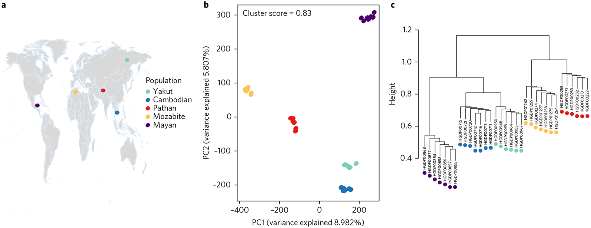
Fig. 1 |. Context of genome-wide population structure.

a, The geographic locations of populations in the data set, shown on a Gall–Peters projection map. b, PCA on the SNP genotype matrix. The first and second PCs explain 9% and 6% of the variation, respectively, and clearly differentiate the individuals into five well-separated clusters that correspond to the five populations sampled. c, A hierarchical clustering tree also captures the genetic relationships between the individuals and their populations.
