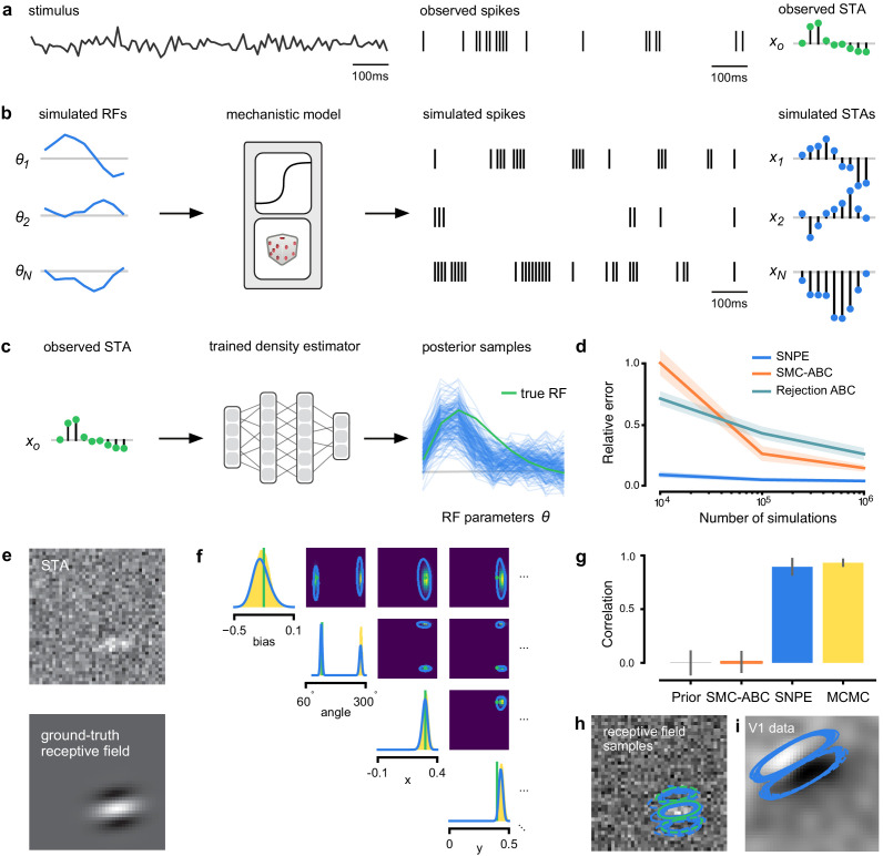
Figure 2. Estimating receptive fields in linear-nonlinear models of single neurons with statistical inference.

(a) Schematic of a time-varying stimulus, associated observed spike train and resulting spike-triggered average (STA) (b) Sequential Neural Posterior Estimation (SNPE) proceeds by first randomly generating simulated receptive fields θ, and using the mechanistic model (here an LN model) to generate simulated spike trains and simulated STAs. (c) These simulated STAs and receptive fields are then used to train a deep neural density estimator to identify the distribution of receptive fields consistent with a given observed STA ${\mathbf{𝐱}}_o$. (d) Relative error in posterior estimation of SNPE and alternative methods (mean and 95% CI; 0 corresponds to perfect estimation, one to prior-level, details in Materials and methods). (e) Example of spatial receptive field. We simulated responses and an STA of an LN-model with oriented receptive field. (f) We used SNPE to recover the distribution of receptive-field parameters. Univariate and pairwise marginals for four parameters of the spatial filter (MCMC, yellow histograms; SNPE, blue lines; ground truth, green; full posterior in Appendix 1—figure 4). Non-identifiabilities of the Gabor parameterization lead to multimodal posteriors. (g) Average correlation (± SD) between ground-truth receptive field and receptive field samples from posteriors inferred with SMC-ABC, SNPE, and MCMC (which provides an upper bound given the inherent stochasticity of the data). (h) Posterior samples from SNPE posterior (SNPE, blue) compared to ground-truth receptive field (green; see panel (e)), overlaid on STA. (i) Posterior samples for V1 data; full posterior in Appendix 1—figure 6.